↗ OpenReview ↗ NeurIPS Homepage ↗ Chat
TL;DR#
Monocular depth estimation (MDE) is a challenging computer vision problem with many applications but existing methods often struggle with local correlation modeling and lack a holistic approach. Many current methods predict depth pixel by pixel without considering relationships between nearby pixels, leading to inaccuracies and inefficient processing. This also ignores the holistic scene context that impacts depth predictions.
DCDepth tackles this by working in the frequency domain, utilizing the Discrete Cosine Transform (DCT). This separates depth information into different frequency components that relate to global structure (low frequency) and fine details (high frequency). A progressive prediction approach is used, starting with low-frequency components to establish scene context and then iteratively adding higher-frequency details. This progressive, frequency-domain approach improves estimation accuracy and efficiency. The method also includes a DCT-inspired downsampling technique to improve information fusion across different scales. Extensive experiments demonstrate that DCDepth achieves state-of-the-art performance on multiple standard datasets.
Key Takeaways#
Why does it matter?#
This paper is important because it presents a novel approach to monocular depth estimation, a crucial task in computer vision with broad applications. By shifting the estimation from the spatial to the frequency domain using DCT, it addresses limitations of existing methods, improving accuracy and efficiency. This opens avenues for future research in progressive estimation strategies and frequency-domain processing for computer vision tasks.
Visual Insights#
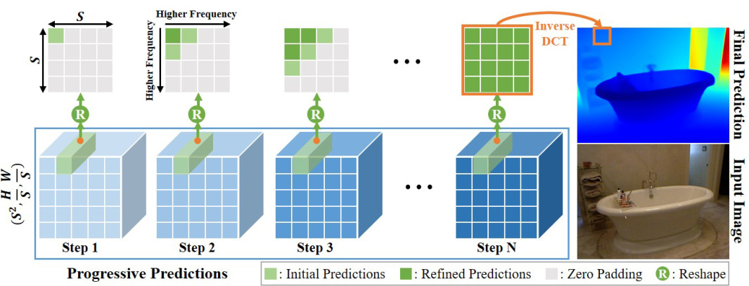
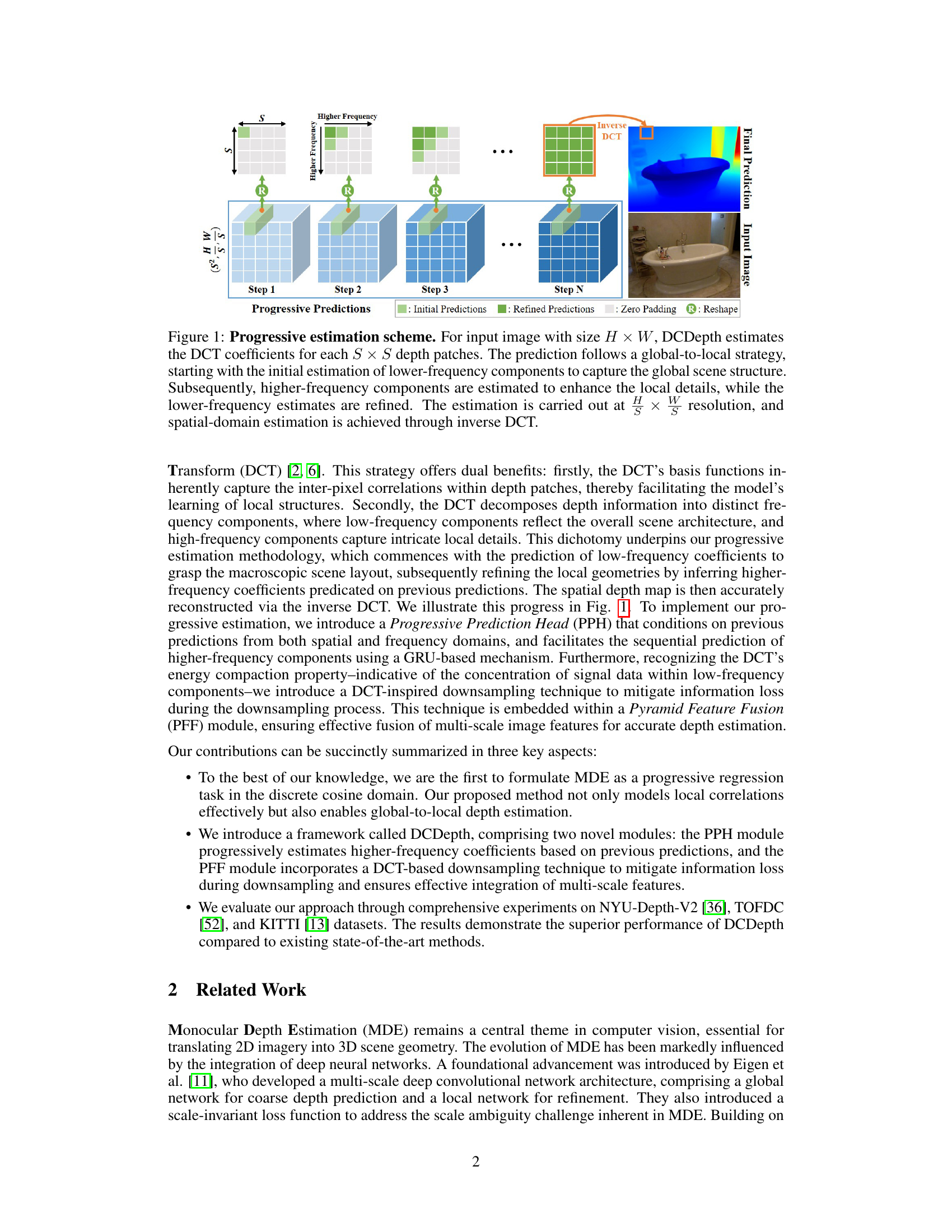
This figure illustrates the progressive depth estimation process used in DCDepth. The input image is divided into SxS patches, and their DCT coefficients are predicted progressively, starting with low-frequency components to establish the global structure and then iteratively refining the prediction with higher-frequency components to add finer details. The process continues until all frequency components are predicted, after which inverse DCT reconstructs the final depth map.
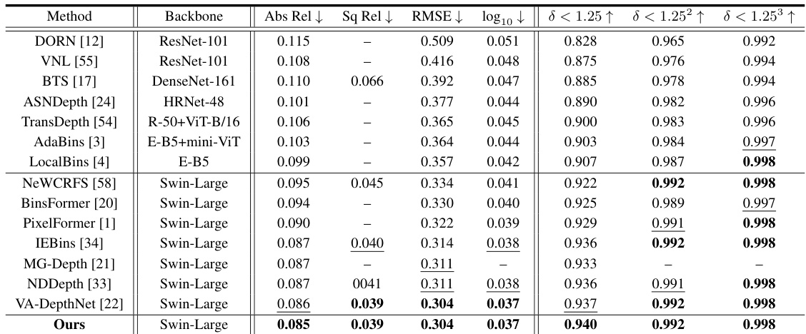
This table presents a quantitative comparison of different monocular depth estimation methods on the NYU-Depth-V2 dataset. It shows several metrics, including absolute relative error (Abs Rel), squared relative error (Sq Rel), root mean squared error (RMSE), log10 error, and three threshold accuracy metrics (δ < 1.25, δ < 1.252, δ < 1.253). The table allows for a comparison of the performance of various methods, indicating their accuracy in depth estimation. Note that the best performing method for each metric is highlighted in bold and the second best is underlined.
In-depth insights#
DCT Depth Estimation#
Discrete Cosine Transform (DCT)-based depth estimation offers a compelling alternative to traditional spatial-domain approaches. By transforming depth map patches into the frequency domain, DCT leverages its energy compaction property, concentrating crucial information in low-frequency components. This allows for a progressive estimation strategy, prioritizing global scene structure before refining local details, improving efficiency and accuracy. Local depth correlations are implicitly captured by DCT’s basis functions, enhancing model learning. The frequency decomposition facilitates a multi-scale representation, enabling effective fusion of both low and high-frequency components for robust depth prediction. However, challenges remain in handling missing or sparse data, common in real-world scenarios, where the DCT’s energy compaction may lead to information loss. Further research is crucial to optimizing the DCT-based methods for sparse datasets and exploring the potential limitations of reliance on purely DCT-based features for depth prediction in highly textured regions. Combining DCT with other techniques may yield superior results.
Progressive Prediction#
Progressive prediction, in the context of a depth estimation model, is a powerful technique that leverages a sequence of predictions to progressively refine the depth map. It starts by predicting low-frequency components to establish a coarse global structure. Then, it iteratively predicts higher-frequency components, integrating them with the previous predictions to progressively refine the local details. This approach is particularly effective because it leverages the inherent structure in the frequency domain of the depth patches; low-frequency components capture the overall scene structure, while high-frequency components represent finer details. This progressive strategy, thus, tackles the inherent ill-posed nature of depth estimation from a single image by decomposing the problem into manageable subproblems. Furthermore, a progressive prediction head may use recurrent neural network structures (e.g. GRU) to maintain a history of previous predictions, thus effectively enabling the model to learn refined and contextually aware representations. The resulting accuracy improvements stem directly from this ability to effectively integrate global and local context, thereby avoiding artifacts associated with independently predicting pixel-wise depth. The efficiency of the method might also be improved using the energy compaction property of the Discrete Cosine Transform (DCT), which tends to concentrate most of the signal’s energy in low-frequency coefficients. This implies potential for effective downsampling techniques that improve computational performance without significant loss of information.
Pyramid Feature Fusion#
Pyramid Feature Fusion (PFF) modules are designed to effectively integrate multi-scale image features for enhanced depth estimation. The core idea is to leverage the complementary information present at different resolution levels, where shallow features capture fine details and deep features provide global context. A critical component of PFF is the proposed DCT-based downsampling technique, which aims to minimize information loss during downscaling, a common challenge with traditional methods. By employing the energy compaction property inherent in the Discrete Cosine Transform (DCT), PFF concentrates crucial signal data, making downsampling more efficient. The fused features are then processed by the decoder for depth map reconstruction. This approach of combining multi-scale features via a carefully designed downsampling strategy is a key innovation, demonstrating an improved depth estimation accuracy compared to traditional approaches which often struggle to efficiently fuse information from multiple resolution levels. The effectiveness of this module is supported by ablation studies showing significant performance improvements when using DCT-based downsampling compared to alternative methods.
Frequency Domain MDE#
The concept of “Frequency Domain MDE” (Monocular Depth Estimation) presents a novel approach to a long-standing computer vision challenge. Instead of directly processing pixel-wise depth information in the spatial domain, this method leverages a frequency transformation, such as the Discrete Cosine Transform (DCT), to represent depth data in terms of frequency components. This has several potential advantages. Lower frequencies capture the overall scene structure, allowing for efficient global context modeling. Higher frequencies encode finer details, enabling progressive refinement. This frequency decomposition also inherently captures local depth correlations within patches, as frequency basis functions naturally encode spatial relationships. A progressive estimation strategy, starting with low frequencies and iteratively refining with higher ones, is particularly well-suited for this frequency representation. Such an approach could lead to significant improvements in computational efficiency and depth estimation accuracy compared to traditional spatial-domain methods, especially in complex scenes with intricate details and sharp depth discontinuities. However, challenges remain, particularly regarding the effective handling of high-frequency components and the development of appropriate loss functions in the frequency domain. Further research is needed to fully explore the potential and limitations of this promising paradigm.
DCDepth Limitations#
The core limitation of DCDepth lies in its reliance on the Discrete Cosine Transform (DCT) for depth estimation. While DCT effectively captures local correlations and separates frequencies, it inherently assumes a piecewise smooth depth structure within patches, which may not always hold true in real-world scenes with sharp discontinuities. This assumption could lead to inaccuracies in depth prediction, particularly in regions with complex geometries or fine details. The progressive refinement strategy, although effective in enhancing global scene context, might still struggle with recovering high-frequency details that are strongly correlated across patches. The method’s dependence on DCT also suggests a limited ability to generalize to diverse image content beyond the datasets used for training. The computational cost associated with repeated DCT and inverse DCT operations across multiple frequency bands could be substantial, potentially limiting real-time applications. Finally, the success of DCDepth heavily depends on the accuracy of initial low-frequency estimations, as errors in the global structure will propagate through subsequent refinement stages.
More visual insights#
More on figures

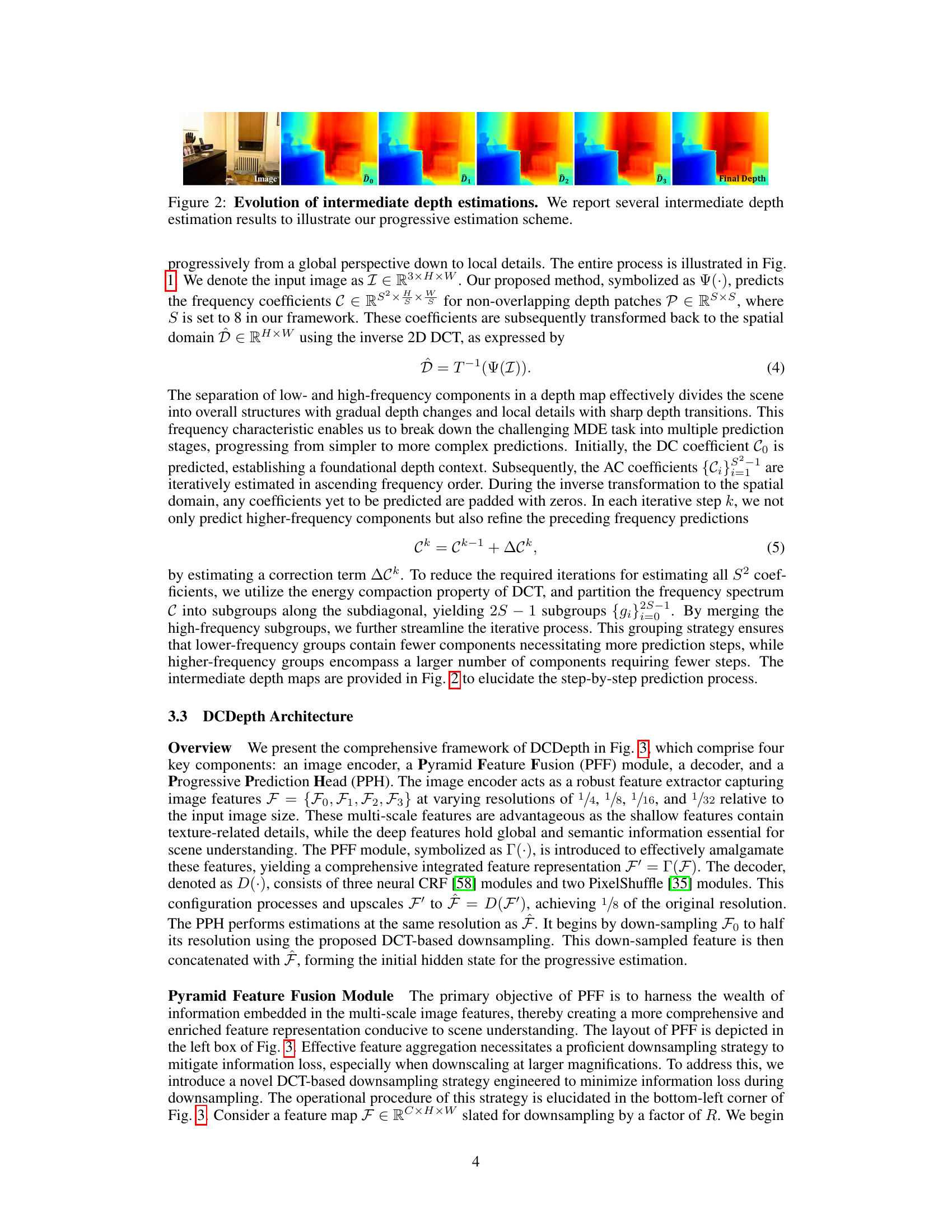
This figure shows the intermediate depth estimation results at different stages of the progressive estimation process. Starting from an initial global prediction (D0), the model refines the depth map iteratively by predicting higher-frequency components (D1, D2, D3), ultimately arriving at the final depth map. This visually demonstrates the progressive nature of DCDepth’s depth estimation, going from coarse to fine detail.
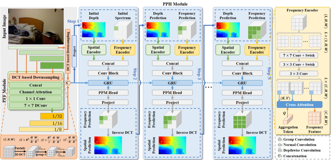
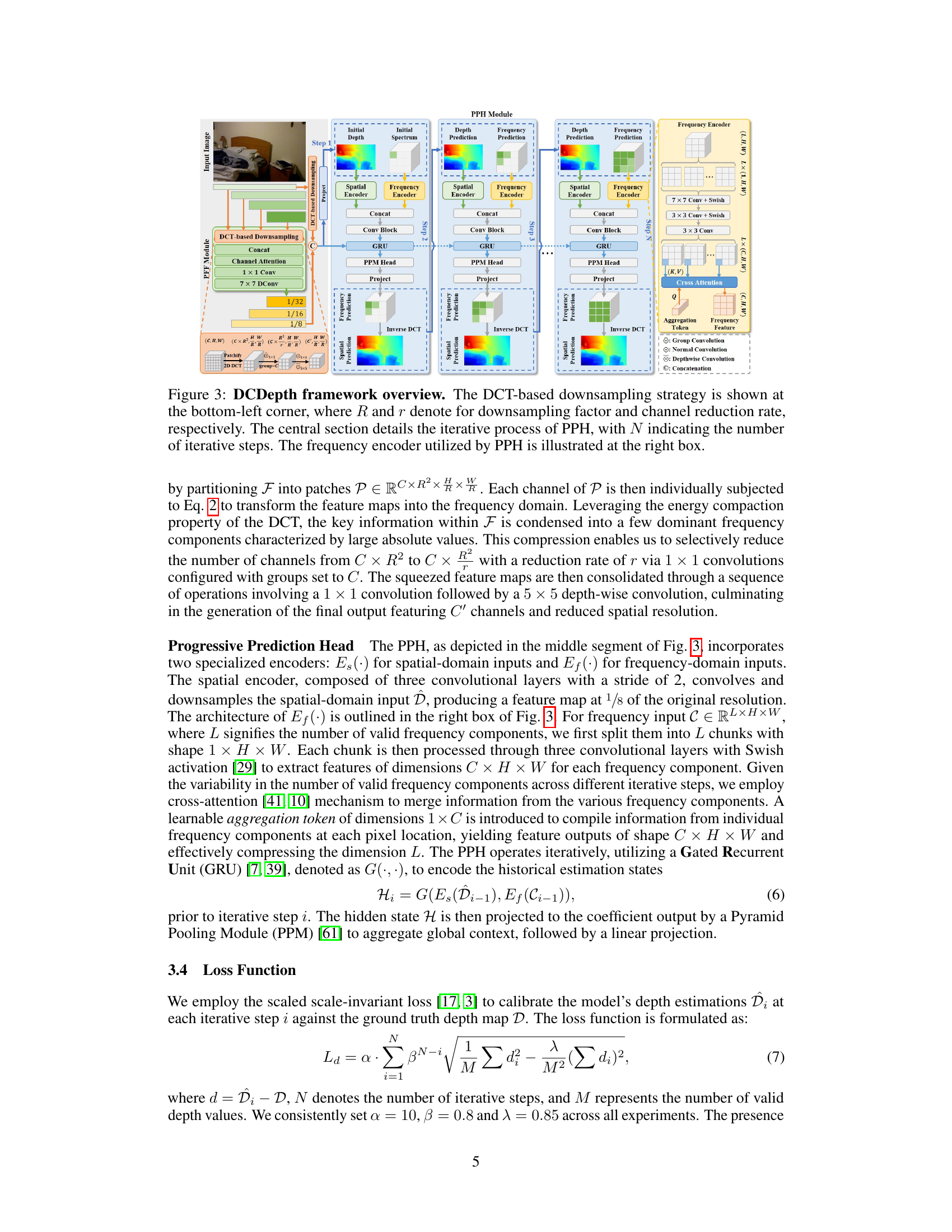
This figure provides a comprehensive overview of the DCDepth framework, highlighting its key components: DCT-based downsampling, Pyramid Feature Fusion (PFF) module, Progressive Prediction Head (PPH) module, and the iterative prediction process. The DCT-based downsampling strategy is shown in detail, emphasizing its role in reducing computational cost and maintaining information. The PPH module’s iterative process, involving both spatial and frequency encoders, is visualized, showing how it progressively refines depth estimations. The figure clearly illustrates the flow of information through each module and the overall architecture of the model.
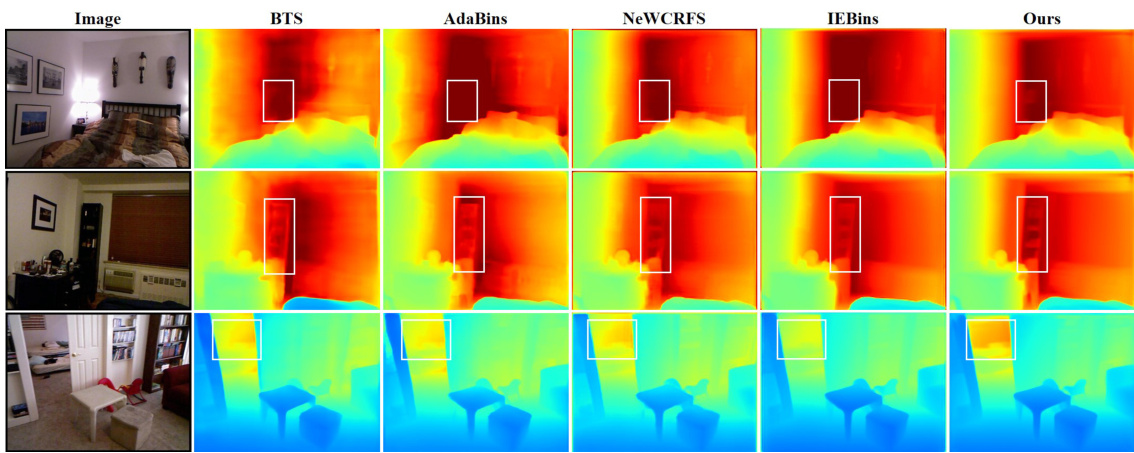
This figure shows a qualitative comparison of depth estimation results on the NYU-Depth-V2 dataset for different methods: BTS, AdaBins, NeWCRFS, IEBins, and the proposed method (Ours). Each row represents a different input image from the dataset. The color scale in the depth maps ranges from blue (closest) to red (farthest). The white boxes highlight areas where the proposed method produces notably more accurate depth estimations compared to other methods, demonstrating its improved performance in capturing fine-grained details and smoothness in planar regions.

This figure shows a qualitative comparison of depth estimation results on the NYU-Depth-V2 dataset, comparing several state-of-the-art methods with the proposed DCDepth method. Two example images are shown with their corresponding depth maps generated by each method. The white boxes highlight areas where the DCDepth method provides noticeably more accurate depth estimates compared to the other approaches. This visual comparison illustrates the enhanced accuracy and detail preservation capabilities of the proposed method in complex scenes with varying depths and textures.

This figure presents a qualitative comparison of depth estimation results on the Eigen split of the KITTI dataset. It shows three methods: AdaBins, NeWCRFS, and the proposed DCDepth method. For each method, the depth map is shown alongside the input image, highlighting the differences in depth prediction accuracy and detail. White boxes indicate regions where DCDepth offers superior performance.

This figure shows the trade-off between accuracy and inference speed as the number of iterative steps in the DCDepth model increases. The y-axis represents the Root Mean Squared Error (RMSE) in centimeters, a measure of prediction accuracy, while the x-axis indicates the number of iterations. The size of each bubble is proportional to the processing time, visually representing the computational cost at each iteration level. The results demonstrate that as the number of iterations increases, accuracy improves but processing time also increases. The figure provides a way to find the optimal balance between these two factors.
More on tables

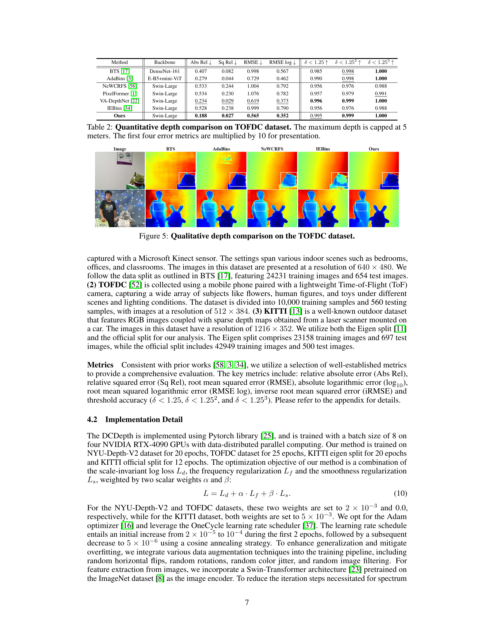
This table presents a quantitative comparison of different monocular depth estimation methods on the TOFDC dataset. It shows the performance of various methods using standard metrics such as Absolute Relative Error (Abs Rel), Squared Relative Error (Sq Rel), Root Mean Squared Error (RMSE), and Root Mean Squared Logarithmic Error (RMSE log). Additionally, it includes threshold accuracy metrics (δ < 1.25, δ < 1.25², δ < 1.25³) to evaluate the accuracy of depth predictions. The maximum depth considered is 5 meters, and the first four error metrics are multiplied by 10 for better presentation.

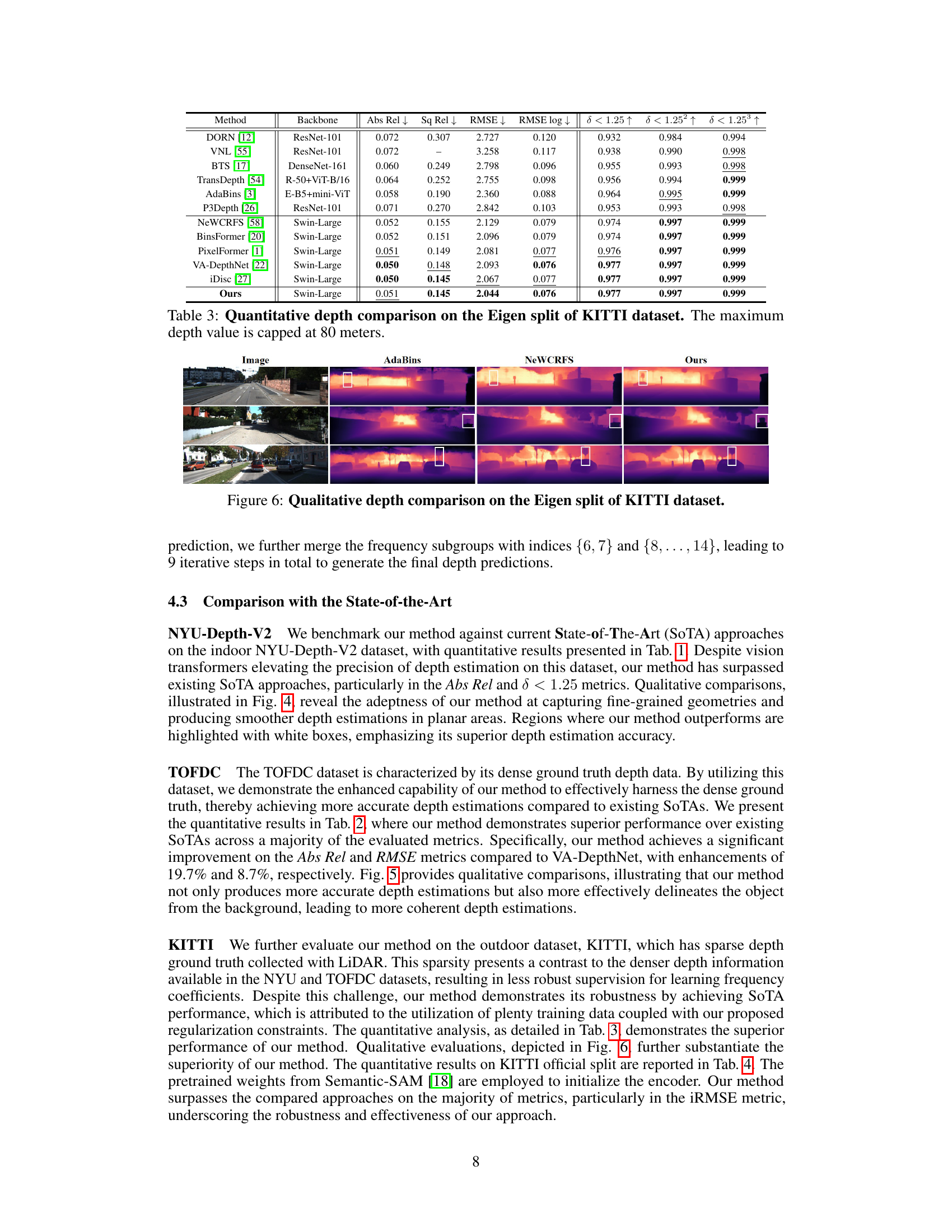
This table presents a quantitative comparison of different monocular depth estimation methods on the Eigen split of the KITTI dataset. The metrics used for comparison include: relative absolute error (Abs Rel), relative squared error (Sq Rel), root mean squared error (RMSE), absolute logarithmic error (log10), and three threshold accuracy metrics (δ < 1.25, δ < 1.25², δ < 1.25³). The maximum depth considered in the evaluation is 80 meters. The table allows readers to directly compare the performance of DCDepth against other state-of-the-art methods on a challenging outdoor dataset known for its sparse depth ground truth.

This table presents a quantitative comparison of different monocular depth estimation methods on the NYU-Depth-V2 dataset. The metrics used to evaluate performance include absolute relative error, squared relative error, root mean squared error, logarithmic error, and three threshold accuracy measures (δ < 1.25, δ < 1.252, δ < 1.253). The table compares the performance of DCDepth against several state-of-the-art approaches. The best performing method for each metric is highlighted in bold, indicating the superior performance of DCDepth.

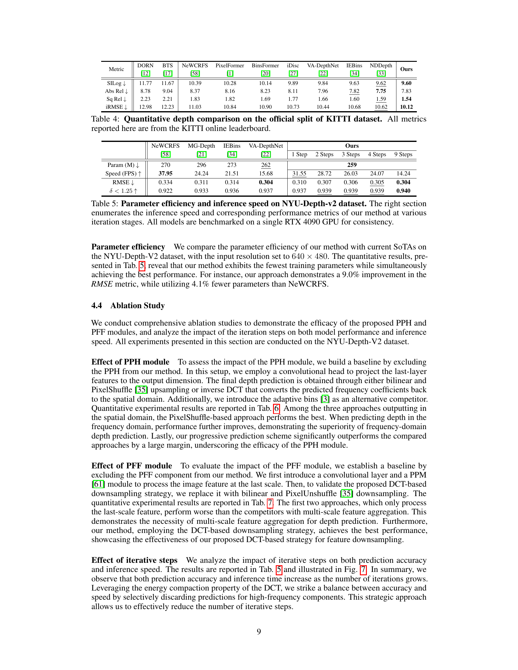
This table compares the parameter efficiency and inference speed of the proposed DCDepth model with several state-of-the-art methods on the NYU-Depth-V2 dataset. It shows the number of parameters (in millions), frames per second (FPS), root mean squared error (RMSE), and the threshold accuracy (δ < 1.25) for each model. The right side of the table specifically illustrates how the performance and speed of DCDepth changes with varying numbers of iterative steps in its progressive estimation process.

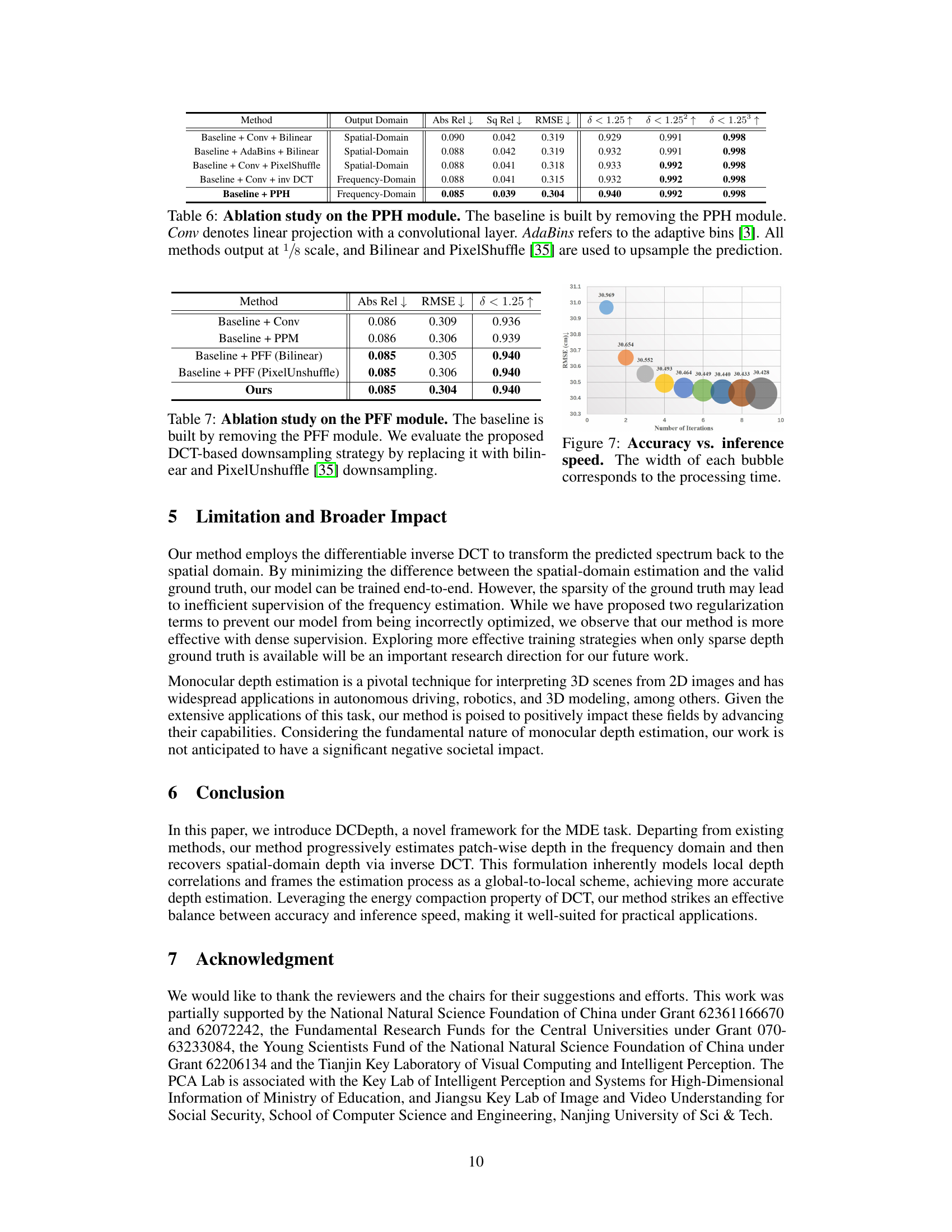
This table presents the ablation study results focusing on the Progressive Prediction Head (PPH) module within the DCDepth framework. It compares different variations of the model, including baselines without the PPH, baselines with different upsampling methods (bilinear and PixelShuffle), and the frequency-domain and spatial-domain outputs. The results demonstrate the effectiveness of the PPH module in improving depth estimation accuracy.

This table presents the results of an ablation study focusing on the Pyramid Feature Fusion (PFF) module within the DCDepth framework. It compares different downsampling strategies (bilinear, PixelUnshuffle, and the proposed DCT-based method) and assesses their impact on the model’s performance. The baseline represents the model without the PFF module, highlighting the contribution of the PFF and the effectiveness of the DCT-based downsampling approach.
Full paper#

