↗ OpenReview ↗ NeurIPS Homepage ↗ Chat
TL;DR#
Recurrent Neural Networks (RNNs) are powerful tools for processing sequential data, but training them effectively remains a challenge. Traditional explanations have focused on vanishing and exploding gradients, but this paper argues that there’s another key obstacle: the “curse of memory.” As RNNs are designed to remember more information, their internal representations become incredibly sensitive to even minor changes in their parameters, which makes effective training incredibly difficult. This sensitivity arises even when gradient issues are addressed.
This research delves into the optimization difficulties faced when training RNNs with long-term dependencies. The authors demonstrate that the complexity of optimization grows exponentially with the memory length of the network, even with stable dynamics. They offer a new understanding of RNN limitations, focusing on signal propagation and its sensitivity to parameter updates. Importantly, they show that architectures like deep state-space models (SSMs) successfully mitigate this “curse of memory” via element-wise recurrence and careful parameterization. This sheds new light on why some RNN architectures outperform others, offering valuable guidance for future research.
Key Takeaways#
Why does it matter?#
This paper is crucial because it challenges the common assumption that solving vanishing/exploding gradients in recurrent neural networks (RNNs) is sufficient for effective long-term memory learning. It introduces the “curse of memory”, a novel problem highlighting increased parameter sensitivity as memory lengthens. This discovery significantly advances our understanding of RNN training difficulties, impacting future model designs and optimization strategies. The findings also stimulate further research into efficient long-sequence learning.
Visual Insights#

This figure shows how the optimization of recurrent neural networks becomes more difficult as their memory capacity increases. Panel A illustrates how changes in network parameters lead to increasingly large output variations as memory increases. Panels B and C demonstrate this phenomenon using a simple one-dimensional teacher-student task, where the loss landscape becomes increasingly sensitive to parameter changes as the memory capacity increases.
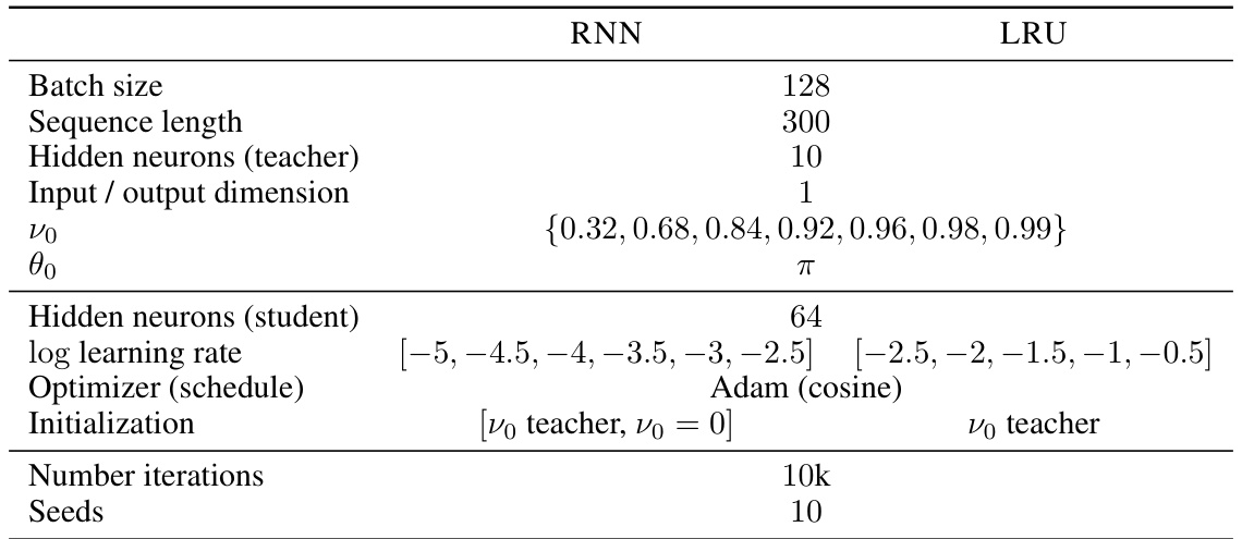
This table details the experimental setup used to generate the results shown in Figure 3.A of the paper. It lists hyperparameters for both RNN and LRU models, including batch size, sequence length, number of neurons, input/output dimensions, and learning rates. It notes that a grid search was performed to find optimal hyperparameters and that the choice to initialize the RNN with vo = 0 yielded better results than initializing with the teacher’s distribution.
In-depth insights#
Memory’s Curse#
The concept of “Memory’s Curse” highlights a critical challenge in training recurrent neural networks (RNNs). While vanishing and exploding gradients hinder learning long-term dependencies, Memory’s Curse reveals a more subtle issue: as a network’s memory increases, even minor parameter changes can lead to vastly different outputs. This extreme sensitivity makes gradient-based optimization incredibly difficult, even if gradients aren’t exploding. The authors propose that careful parametrization and element-wise recurrence, as seen in deep state-space models (SSMs) and LSTMs, are crucial in mitigating this curse. The analysis suggests that the simplicity of SSMs facilitates in-depth analysis, providing insights into how these architectures handle long-range dependencies, overcoming the sensitivity that arises from extended memory. This concept expands our understanding of RNN training difficulties, shifting the focus beyond just gradient issues to include parameter sensitivity which significantly impacts training success.
Linear RNN Limits#
The limitations of linear recurrent neural networks (RNNs) stem from their inherent inability to effectively capture long-range dependencies in sequential data. Linearity restricts the model’s capacity to learn complex temporal dynamics, making it struggle with tasks requiring the integration of information across extended time intervals. The vanishing gradient problem, while significantly mitigated by various architectural innovations, still poses a challenge, particularly in scenarios where the network attempts to model long-term dependencies. The curse of memory emerges as another key limitation, where increased sensitivity to parameter changes arises with longer memory horizons. This sensitivity leads to more complex loss landscapes that significantly hinder optimization, even when gradient explosion is controlled. Addressing these challenges requires a shift toward more sophisticated architectures such as deep state-space models (SSMs) or gated RNNs (like LSTMs and GRUs). These models employ techniques like normalization and reparametrization to improve training stability and alleviate sensitivity to parameter updates, thereby enhancing their ability to capture long-term dependencies. While the simplicity of linear RNNs offers analytical tractability, their limitations highlight the need for more expressive architectures when dealing with complex sequential data.
Diagonal Benefits#
The concept of “Diagonal Benefits” in the context of recurrent neural networks (RNNs) centers on the architectural advantages of using diagonal or near-diagonal weight matrices. This structure offers significant computational efficiency, as matrix multiplication simplifies considerably. Moreover, diagonal RNNs exhibit improved training stability, mitigating the notorious vanishing and exploding gradient problems that plague standard RNNs. This stability arises because diagonal matrices have easily controlled eigenvalues, preventing the exponential growth or decay of error signals during backpropagation. Consequently, optimization becomes less sensitive to parameter changes, reducing the risk of the loss landscape becoming overly sharp. The impact is not solely on training: diagonal structures often lead to faster inference speeds, reducing the computational burden when making predictions. However, it’s crucial to acknowledge that limiting the connectivity to a diagonal pattern may restrict the network’s expressiveness, possibly sacrificing its ability to capture complex dependencies within sequential data. The trade-off is between computational efficiency and representational capacity, which needs to be carefully considered when designing RNN architectures for specific tasks and datasets.
Adaptive Learning#
The concept of adaptive learning rates in the context of recurrent neural networks (RNNs) is crucial for mitigating the challenges posed by the “curse of memory.” Standard optimization algorithms often struggle with RNNs due to the sensitivity of long-term dependencies to parameter updates. Adaptive learning methods dynamically adjust learning rates based on the loss landscape, potentially resolving issues arising from exploding or vanishing gradients. This approach is particularly relevant when dealing with RNN architectures that exhibit a complex loss landscape, characterized by regions of high sensitivity and flat regions. The paper’s exploration into diagonal connectivity, eigenvalue reparametrization, and input normalization are all attempts to improve the conditioning of the loss surface, making it more amenable to adaptive learning strategies. This suggests a synergy between architectural design and optimization techniques, implying that careful design choices can significantly improve the efficacy of adaptive learning in training complex recurrent models.
Deep RNNs#
Deep Recurrent Neural Networks (RNNs) present a fascinating challenge in deep learning. While the theoretical understanding of standard RNNs is hampered by the vanishing/exploding gradient problem, deep architectures introduce a new layer of complexity: the sensitivity to parameter changes increases exponentially with depth, even without gradient explosions. This phenomenon, termed the “curse of memory,” arises from the repeated application of the same update function across many time steps. Careful parametrization and normalization strategies are crucial to mitigate this issue. Deep state-space models (SSMs) and gated RNNs like LSTMs and GRUs exemplify successful approaches by incorporating mechanisms that effectively control the sensitivity of the hidden states. Diagonal recurrent connectivity plays a key role in managing this sensitivity, improving the conditioning of the loss landscape and enabling the use of adaptive learning rates. However, fully connected deep RNNs remain significantly harder to train due to the complex interactions between parameters. Further research is needed to fully understand and address these challenges in training deep RNNs and unlock their potential for handling long-range dependencies effectively.
More visual insights#
More on figures

The figure visualizes how the optimization of recurrent neural networks becomes more challenging as their memory capacity increases. Panel A shows the evolution of the second moment of the derivative of hidden states (dλht) with respect to a recurrent parameter (λ) as a function of λ and the input auto-correlation decay rate (ρ). As the memory increases (λ → 1), the sensitivity of ht to changes in λ also increases, especially when inputs are more correlated (ρ → 1). This increased sensitivity makes gradient-based learning difficult, even without exploding gradients. Panels B and C illustrate this phenomenon in a simple one-dimensional teacher-student task, showing the loss landscapes become sharper and optimization more difficult as the memory capacity of the student network increases.

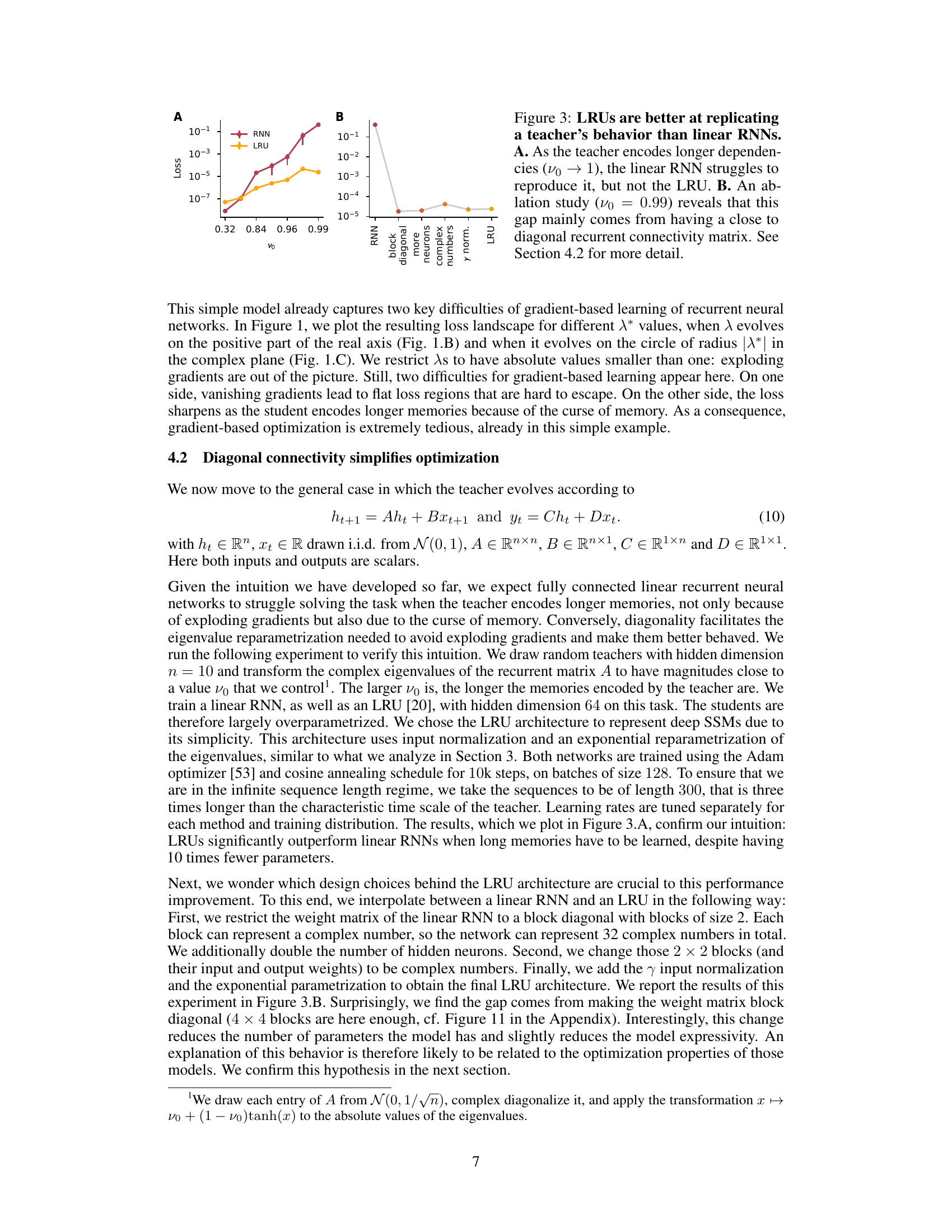
This figure compares the performance of Linear Recurrent Units (LRUs) and Recurrent Neural Networks (RNNs) on a teacher-student task where the teacher model encodes increasingly long-term dependencies, controlled by the parameter νο. Panel A shows that as the temporal dependence increases (νο approaches 1), the RNN’s performance significantly degrades, while the LRU maintains good performance. Panel B investigates what aspects of the LRU architecture contribute to its superior performance, through an ablation study with νο = 0.99. It finds that a key factor is the near-diagonal nature of its recurrent connectivity matrix. The results highlight the challenges faced by standard RNNs in learning long-range dependencies and the effectiveness of LRU’s design in mitigating these challenges.

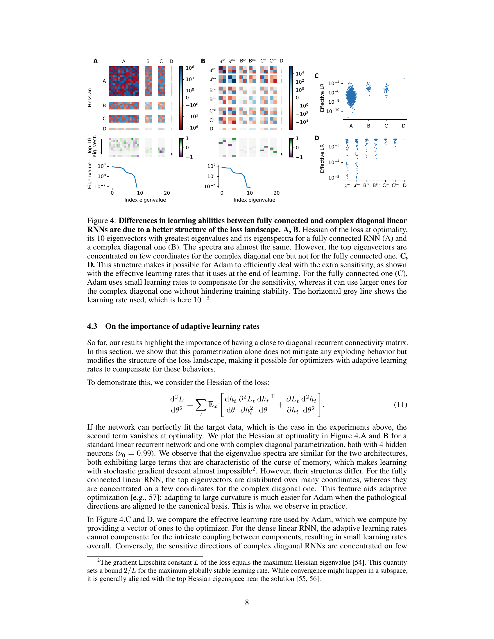
This figure compares the Hessian matrices of the loss function at optimality for fully connected and complex diagonal linear RNNs. It shows that while the eigenvalue spectra are similar, the top eigenvectors are concentrated on fewer coordinates for the complex diagonal RNN, making it easier for the Adam optimizer to handle sensitivity issues and use higher learning rates. The fully connected RNN, in contrast, requires smaller learning rates due to the less structured Hessian.

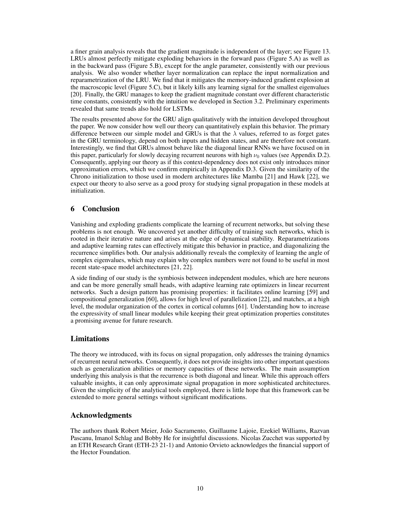
This figure shows the results of an experiment to analyze signal propagation in deep recurrent neural networks at initialization. Panel A shows that input normalization in LRUs and GRUs keeps neural activity constant across different values of the exponential decay parameter (vo). Panel B compares the evolution of loss gradients for different recurrent network types; only the angle of parameter λ explodes for LRUs, while GRUs maintain controlled gradients. Panel C demonstrates that layer normalization controls overall gradient magnitude in complex-valued RNNs. The results support the paper’s theory of signal propagation.
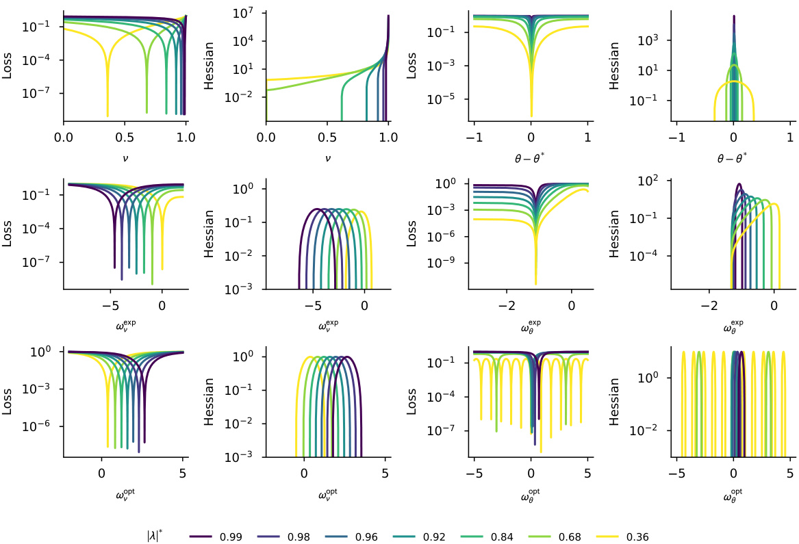
This figure visualizes the loss landscape for a one-dimensional recurrent neural network for various parameterizations (polar, exponential, and optimal). It demonstrates how the loss landscape changes as the teacher’s memory (represented by |λ*|) increases. The plot highlights the impact of different parametrizations on controlling Hessian explosion and the size/number of basins of attraction around optimality, especially emphasizing the difficulty in learning the angle parameter.
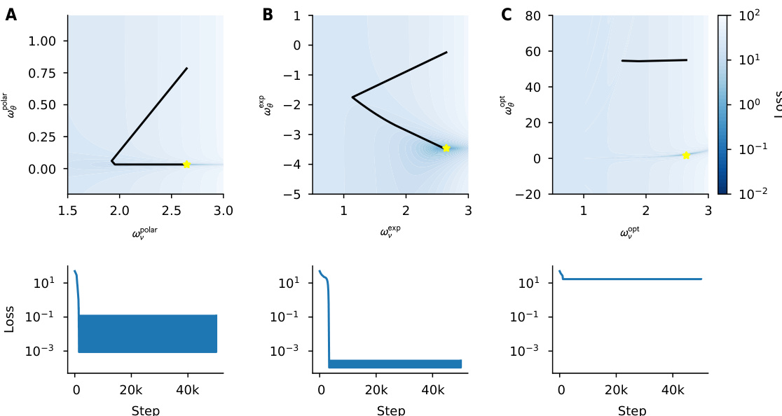
This figure shows how different parametrizations of the recurrent weight (λ) affect the loss landscape for a simple 1D recurrent network. The plots illustrate the loss as a function of the magnitude and angle of λ, for different values of the teacher’s recurrent weight (λ*). The results show how input normalization and reparametrization strategies help to mitigate issues with the loss landscape (e.g., sharp gradients), which are particularly apparent when trying to learn long-term dependencies (|λ*| close to 1). The optimal parametrization reduces the sharpness near the optimum but makes optimization more challenging away from the optimum.

This figure visualizes the magnitude of the function S(λ, λ₀, ρ) across different values of λ (represented on a complex plane), for a fixed λ₀ = 0.99 exp(ίπ/4) and different values of ρ (representing the autocorrelation of inputs). The function S(λ, λ₀, ρ) relates to the Hessian of the loss function, with larger values of |S(λ, λ₀, ρ)| indicating stronger correlations between eigenvalues in the Hessian. The plot shows how this correlation structure changes with the autocorrelation ρ. For uncorrelated inputs (ρ = 0), eigenvalues that are conjugates of each other have large |S(λ, λ₀, ρ)| values. As the correlation increases (ρ approaching 1), this conjugate-related correlation weakens, and the correlation becomes more influenced by eigenvalues approaching 1 in magnitude.

This figure compares the Hessian matrix of the loss function at optimality for fully connected and complex diagonal linear RNNs. The eigenvalue spectra are similar for both architectures, but the eigenvectors differ significantly. In the complex diagonal RNN, top eigenvectors concentrate on a few coordinates, while they are more spread out in the fully connected RNN. This difference in eigenvector structure affects how the Adam optimizer handles the sensitivity of the loss landscape to parameter changes, resulting in the complex diagonal RNN using significantly larger learning rates than the fully connected model.

This figure compares the Hessian of the loss at optimality for fully connected and complex diagonal linear RNNs. While the eigenvalue spectra are similar, the top eigenvectors are concentrated on a few coordinates for the complex diagonal RNN, unlike the fully connected one. This difference in structure allows Adam optimizer to use larger learning rates for the complex diagonal RNN without sacrificing stability, whereas smaller rates are needed for the fully connected RNN to compensate for the increased sensitivity.

This figure shows the impact of the number of heads in a linear recurrent neural network on both the final loss and the effective learning rates. Panel A demonstrates that increasing the number of heads (decreasing the total number of parameters) leads to lower final loss, indicating improved performance. Panel B shows that while increasing the number of heads initially increases the effective learning rate, this trend reverses later in training. This suggests a trade-off between the expressiveness of the model and the efficiency of optimization; more heads initially allow for faster learning, but eventually lead to diminishing returns.
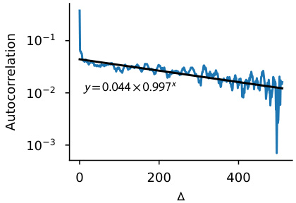
The figure shows the empirical autocorrelation function of BERT embeddings from the Wikipedia dataset. The blue line shows the empirical data, which is approximated by a sum of two exponential decay functions. The black line shows a linear regression approximation of the log autocorrelation.

This figure shows the results of experiments on signal propagation in deep recurrent neural networks at initialization. Panel A shows that input normalization in LRUs and GRUs keeps neural activity constant across different memory lengths. Panel B compares the evolution of loss gradients for different recurrent network types, highlighting the effectiveness of LRUs and GRUs in mitigating gradient explosion. Panel C demonstrates that layer normalization helps control gradient magnitude in complex RNNs.
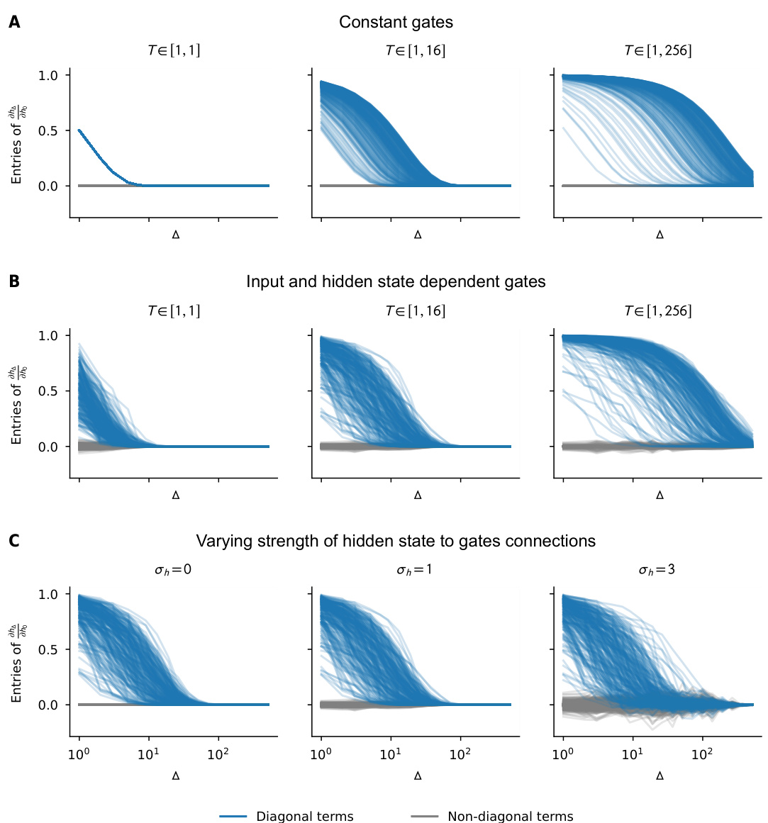
This figure shows the evolution of the recurrent Jacobian in GRUs under different conditions. The results support the claim that GRUs behave similarly to diagonal linear networks, especially when the gates are independent of inputs and hidden states. The impact of varying the strength of the hidden state to gate connections on the Jacobian is also shown.
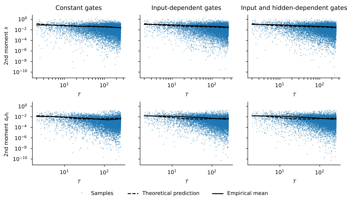
This figure shows the results of an experiment to verify the theory of signal propagation in deep recurrent neural networks at initialization. Panel A shows that input normalization in LRUs and GRUs helps to keep neural activity constant even with long-term dependencies. Panel B demonstrates that the gradients explode in complex diagonal RNNs but are controlled in LRUs and GRUs. Panel C shows that layer normalization helps maintain gradient magnitude in cRNNs.
More on tables

This table details the hyperparameters used in the experiments for Figure 3B. It compares three variations of recurrent neural networks: a standard RNN, a block diagonal RNN (with 2x2 blocks), and a complex diagonal RNN/LRU. The table lists settings for batch size, sequence length, number of neurons (both teacher and student), input/output dimension, the vo parameter (controlling memory length), the learning rate (log scale), optimizer, initialization method, number of training iterations and random seeds.

This table details the experimental setup used to generate the results shown in Figure 10 of the paper. It specifies hyperparameters for both RNN and complex diagonal RNN/LRU models, including batch size, sequence length, number of neurons, input/output dimensions, values of vo and θ0, learning rates, optimizer, initialization methods, number of iterations, and random seeds used. The table highlights the hyperparameter search process and choices made to optimize the experimental conditions.
Full paper#


