↗ OpenReview ↗ NeurIPS Homepage ↗ Chat
TL;DR#
Offline model-based reinforcement learning (MBRL) is promising for data-efficient learning, especially when exploration is costly. However, a major limitation is the objective mismatch between model and policy learning, leading to poor performance. This paper identifies that confounders in offline data are the main cause of this mismatch.
To solve this, the paper introduces BECAUSE, a novel algorithm that learns a causal representation of states and actions. This representation helps to reduce the impact of confounders, leading to improved model accuracy and policy performance. BECAUSE is evaluated on various tasks and demonstrates significantly better generalizability and robustness than existing offline RL methods, especially in low-sample data regimes and in the presence of numerous confounders.
Key Takeaways#
Why does it matter?#
This paper is important because it tackles the crucial problem of objective mismatch in offline model-based reinforcement learning (MBRL), a significant hurdle in improving data efficiency and generalization. By introducing a novel causal representation learning framework (BECAUSE), it offers a potential solution to this challenge, which has implications for various fields where active exploration is expensive or infeasible. The theoretical analysis and empirical evidence presented provide a strong foundation for future research in causal MBRL.
Visual Insights#
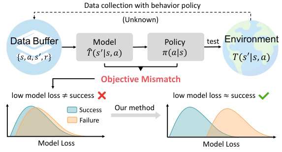
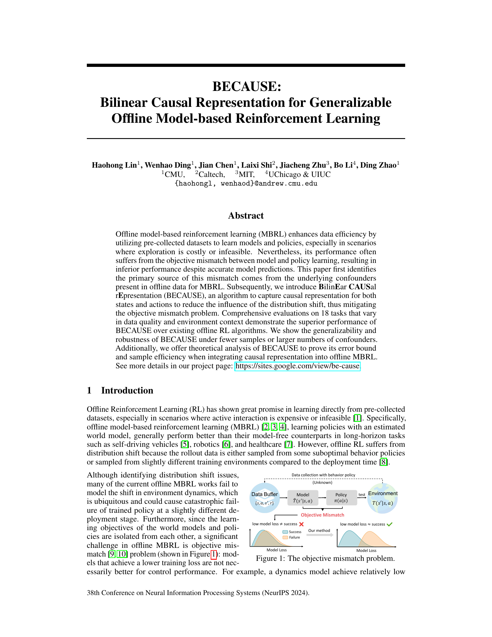
The figure illustrates the objective mismatch problem in offline model-based reinforcement learning (MBRL). In standard offline MBRL, a low model loss doesn’t guarantee successful policy deployment because of a mismatch between the model training objective and the policy’s success. The left panel shows this mismatch: low model loss is not correlated with policy success. The right panel illustrates how the proposed method, BECAUSE, addresses this mismatch by aligning model loss with policy success, improving generalizability.
This table presents the statistical significance tests comparing the performance of the proposed BECAUSE method against 10 baseline methods across 18 different tasks. A p-value is calculated for each comparison, indicating the probability of observing the results if there were no true difference between BECAUSE and the baseline. P-values below 0.05 are considered statistically significant and highlighted in green, indicating that BECAUSE outperforms the baseline.
In-depth insights#
Causal Offline RL#
Causal Offline RL represents a significant advancement in reinforcement learning, aiming to address the limitations of traditional offline RL methods. Standard offline RL struggles with distribution shift, where the data used for training differs from the deployment environment. Causal methods attempt to overcome this by explicitly modeling the causal relationships within the environment. This allows for more robust generalization and improved performance, even with limited data. By disentangling confounding factors, causal offline RL can identify true causal effects and reduce reliance on spurious correlations learned from biased data. This leads to policies that generalize better to unseen situations, enhancing the data efficiency and reliability of offline RL. However, the application of causal inference in offline RL presents significant computational challenges. Accurate causal discovery and representation learning are crucial yet difficult tasks, especially when dealing with complex, high-dimensional environments and limited data. Despite the challenges, the pursuit of causal offline RL holds immense promise for improving the safety and robustness of RL applications in various fields, such as robotics, healthcare, and autonomous systems.
Bilinear MDPs#
Bilinear Markov Decision Processes (MDPs) offer a powerful way to model complex systems by capturing the interaction between states and actions through bilinear forms. This representation is particularly useful in scenarios with high-dimensional state and/or action spaces, where traditional methods might struggle. The bilinear structure allows for a compact and efficient representation, potentially reducing the computational burden of model learning and planning. A key advantage is the ability to factorize the dynamics into separate representations of states and actions, which simplifies modeling and enhances generalizability. By learning low-rank approximations of the bilinear components, one can extract meaningful features and structure from the environment. However, challenges remain in choosing the appropriate feature representations and in ensuring that the bilinear model accurately captures the system dynamics. Further research into robust and efficient learning algorithms for bilinear MDPs is needed to fully unlock their potential.
BECAUSE Algorithm#
The BECAUSE algorithm, designed for generalizable offline model-based reinforcement learning (MBRL), tackles the challenge of objective mismatch. It achieves this by focusing on causal representation learning, identifying and mitigating the influence of confounders present in offline datasets. By approximating causal representations for both states and actions using bilinear MDPs, BECAUSE reduces spurious correlations and distribution shifts. Causal discovery methods help estimate an unconfounded world model, leading to more robust and generalizable policies. Furthermore, BECAUSE incorporates uncertainty quantification, utilizing energy-based models (EBMs) to provide a measure of uncertainty in state transitions, enabling conservative planning and avoiding out-of-distribution (OOD) states. This combination of causal representation learning and uncertainty-aware planning enhances the overall generalizability and robustness of the offline MBRL approach, particularly beneficial in scenarios with limited data or high levels of confounding factors. The theoretical analysis further supports its efficiency and provides error bounds. Empirical results demonstrate BECAUSE’s superiority over various baselines across a range of tasks and datasets, showing its promise in addressing the limitations of traditional offline RL methods.
Generalization Bounds#
Generalization bounds in machine learning offer a crucial theoretical framework for understanding a model’s ability to perform well on unseen data. They provide a quantitative measure of the difference between a model’s performance on the training set and its expected performance on new, unseen data, offering insights into model complexity, data size, and the learning algorithm’s properties. Tighter bounds indicate a better ability to generalize. Factors such as the VC dimension or Rademacher complexity directly relate to the capacity of a model to fit complex functions, and hence influence the generalization bound. Larger datasets and appropriate regularization techniques help narrow the gap between training and test performance, thereby improving generalization and leading to tighter bounds. The quest for tighter bounds often involves balancing model complexity and data size, highlighting a trade-off between model expressiveness and its capacity to generalize. Studying generalization bounds is essential for designing robust and reliable machine learning systems.
Empirical Analysis#
An empirical analysis section in a research paper would typically present the results of experiments designed to test the paper’s hypotheses or claims. A strong empirical analysis would go beyond simply reporting numbers; it would carefully describe the experimental setup, including data sources, participant characteristics (if applicable), and the methods used for data collection and analysis. The analysis would also focus on the key findings relevant to the paper’s central research question, and provide sufficient detail for the reader to understand the results and evaluate their validity. Important considerations include statistical significance, including effect sizes and confidence intervals, and comparisons with relevant baselines or prior work to demonstrate the novelty and impact of the findings. Visualizations (e.g., graphs, tables) should be well-integrated into the narrative and help to clarify the results. Finally, a discussion of any limitations, potential biases, or unexpected findings would enhance transparency and trustworthiness.
More visual insights#
More on figures
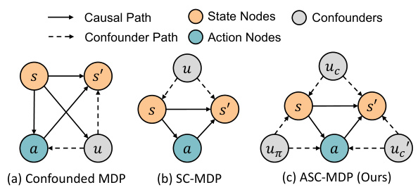
This figure compares three different causal models for Markov Decision Processes (MDPs) with confounders. (a) shows a confounded MDP where confounders affect both the state transition and the relationship between states and actions. (b) shows an SC-MDP (State-Confounded MDP) where confounders only influence the state transition. (c) shows the proposed ASC-MDP (Action-State-Confounded MDP), which models confounders affecting both the state transition and the relationship between states and actions, as well as the correlation between actions and states.

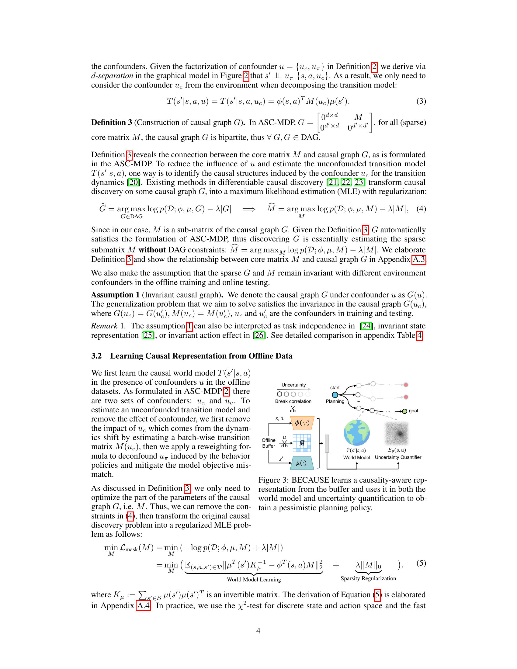
The figure illustrates the BECAUSE framework. It shows how the algorithm learns a causal representation from offline data to improve the generalization and robustness of offline model-based reinforcement learning. The framework consists of three main components: 1. Causal Representation Learning: The offline data buffer is processed using feature mappings φ(.) and μ(.) and the learned causal mask M to obtain a causal representation of states and actions that is less sensitive to confounding factors. 2. World Model: The causal representation is used to learn a more robust and generalizable world model T(s’|s,a) that accurately predicts the next state s’ given the current state s and action a. 3. Uncertainty Quantification: An energy-based model Eg(s, a) is used to quantify the uncertainty of the model’s predictions. This uncertainty is then incorporated into the planning process to make the policy more conservative and less likely to fail in unseen environments. This uncertainty quantification helps mitigate the objective mismatch problem in offline RL.
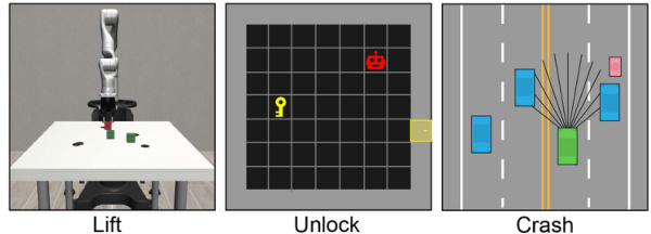
This figure shows three different reinforcement learning environments used in the paper’s experiments. The ‘Lift’ environment involves a robotic arm manipulating objects. The ‘Unlock’ environment is a grid world where an agent must navigate to collect a key and unlock a door. The ‘Crash’ environment simulates an autonomous driving scenario where the agent must avoid collisions with pedestrians and other vehicles.
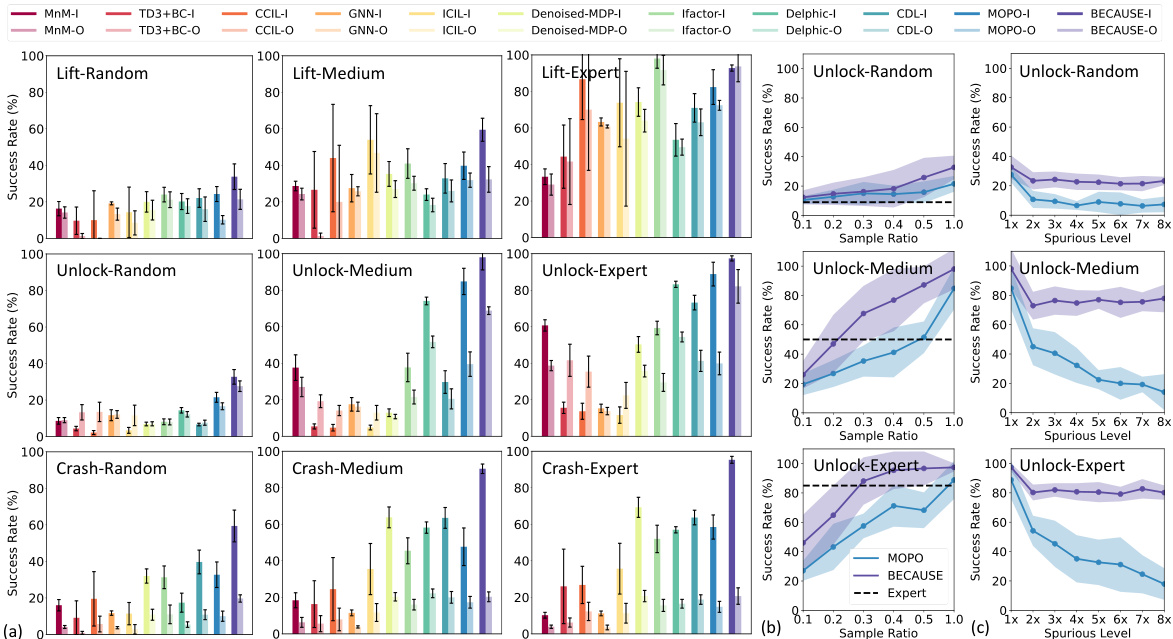
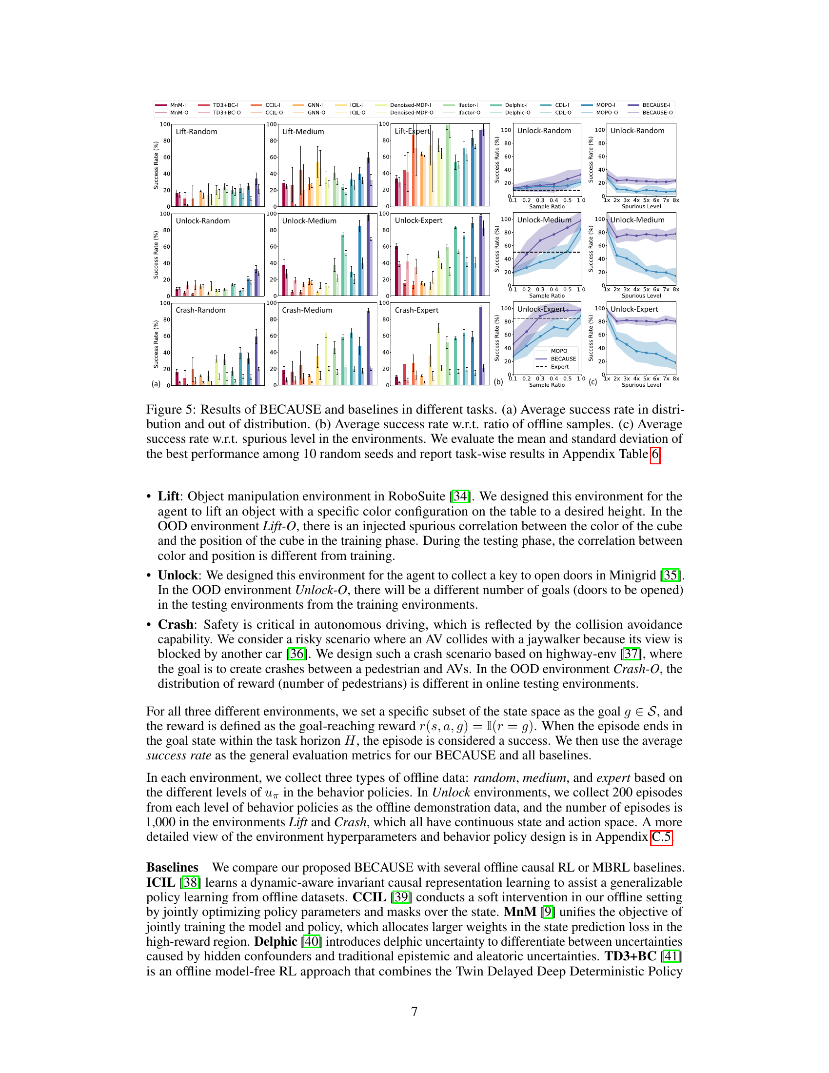
This figure displays the results of the BECAUSE algorithm and its baselines across various tasks. Panel (a) compares the average success rate in distribution and out-of-distribution settings. Panel (b) shows how the success rate changes with varying ratios of offline samples used for training. Panel (c) illustrates the robustness of the algorithms by demonstrating the impact of different spurious correlation levels on the success rate. The results are averaged over 10 trials, and detailed task-wise information can be found in Appendix Table 6.
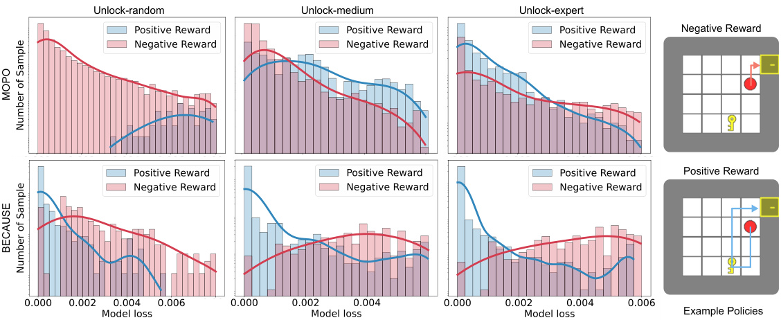
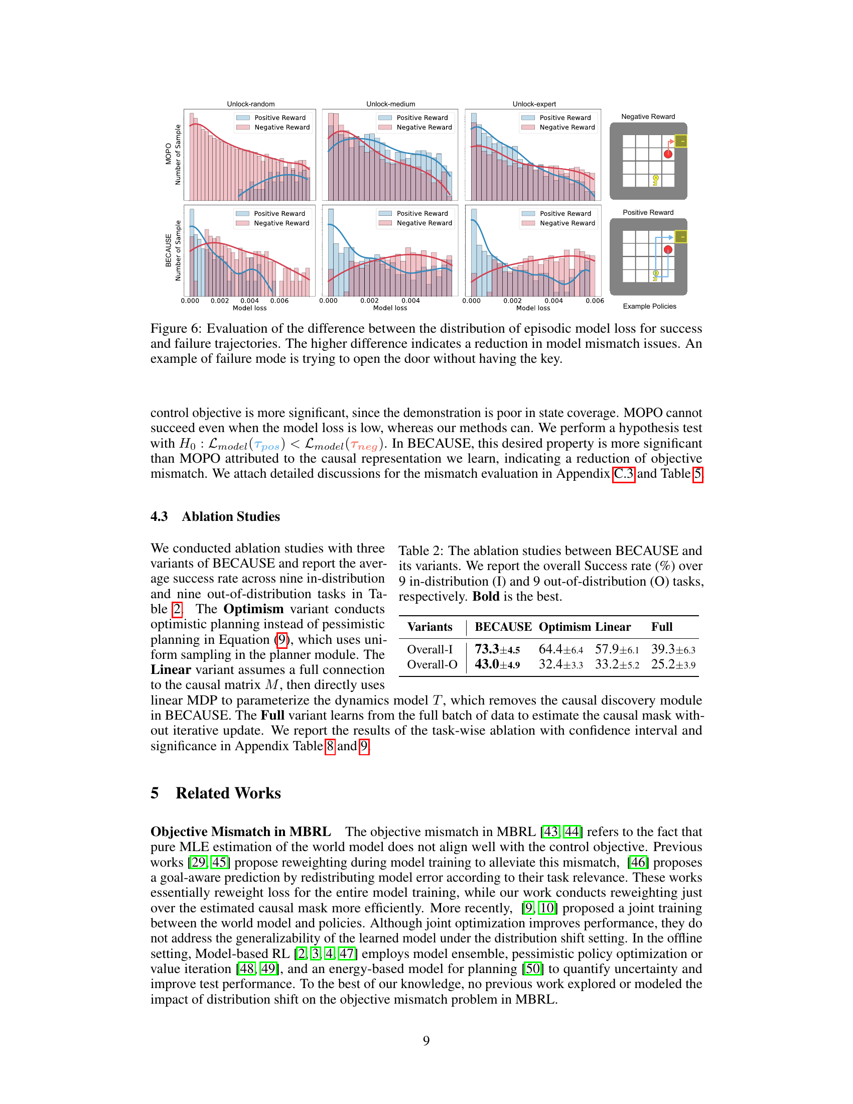
This figure compares the distribution of episodic model loss for successful and failed trajectories in the Unlock environment using two different methods: MOPO and BECAUSE. The x-axis represents the model loss, and the y-axis shows the number of samples. Separate distributions are shown for positive reward (success) and negative reward (failure) trajectories. The key observation is that BECAUSE exhibits a greater separation between the loss distributions for successful and failed trajectories compared to MOPO. This indicates that BECAUSE is better at mitigating the objective mismatch problem, meaning that low model loss more reliably translates into successful outcomes. An example of a failure case is shown in the figure’s inset, where the agent attempts to open a door without possessing the required key. The figure helps to illustrate the performance improvement of BECAUSE by showing that a lower model loss correlates more strongly with success than in the case of MOPO.

This figure compares the convergence speed of two different methods for training an Energy-based Model (EBM) used in the BECAUSE algorithm. The top row shows the training process using randomly sampled negative samples. The bottom row shows the training process using negative samples generated by mixing latent factors from the offline data, a technique leveraging causal representation learned by the BECAUSE algorithm. The images in each row visualize the distribution of the EBM outputs at different timesteps during training. The visualization demonstrates that the causally-informed negative sampling technique leads to faster convergence.

This figure shows the causal graphs learned by BECAUSE for each of the three environments used in the experiments: Lift, Unlock, and Crash. Each graph visually represents the causal relationships between the state and action variables in the respective environment. The nodes represent variables, and edges represent causal relationships. The graphs are bipartite, with one set of nodes representing state variables at a given time step, and the other set representing state variables at the next time step, along with action variables. The sparsity of the graphs highlights the focus on significant causal relationships, ignoring less influential correlations.
More on tables
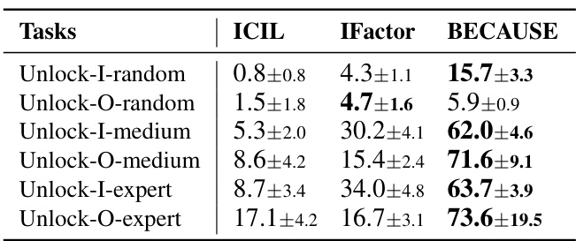
This table compares the performance of ICIL, IFactor, and BECAUSE on visual RL tasks in the Unlock environment. It shows the average success rate for each method across different data quality levels (random, medium, expert) and in-distribution (I) and out-of-distribution (O) settings. BECAUSE consistently demonstrates significantly higher success rates than the baselines, highlighting its superior generalization capabilities in visual scenarios.

This table presents the results of ablation studies comparing the performance of the main proposed method, BECAUSE, against three variants: Optimism, Linear, and Full. The ‘Overall-I’ column shows the average success rate across nine in-distribution tasks (tasks where the testing environment matches the training environment), while ‘Overall-O’ represents the average success rate across nine out-of-distribution tasks (where the testing environment differs from the training one). The bolded values indicate the best performance for each scenario. This demonstrates the importance of each component in the BECAUSE framework for achieving superior performance.

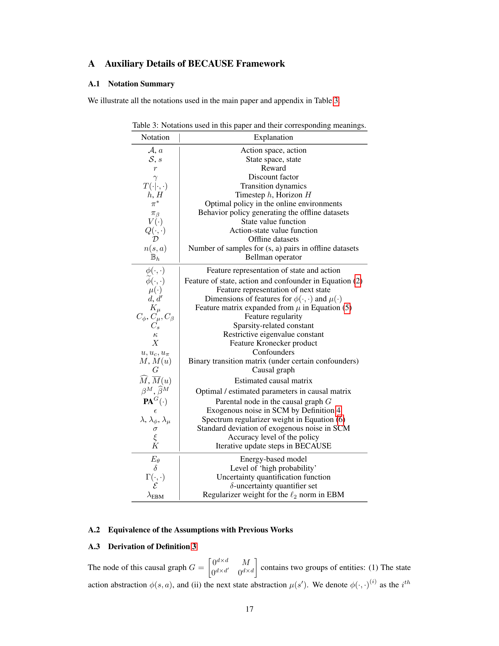
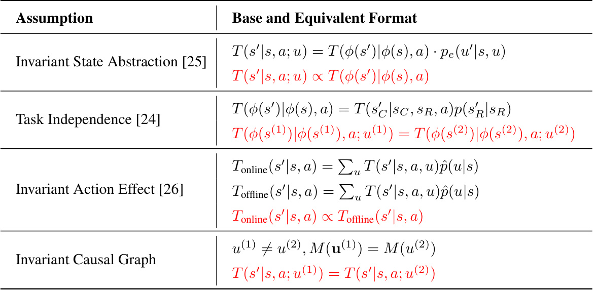
This table lists notations used in the paper and their corresponding meanings. It provides a key to understanding the mathematical symbols and abbreviations used throughout the paper, clarifying the meaning of variables, functions, sets, and other mathematical objects. The table is essential for anyone attempting to reproduce the results or understand the algorithms presented in the paper.
This table presents the statistical significance tests comparing the proposed BECAUSE method against ten baseline methods across eighteen tasks. The p-values indicate whether the performance difference between BECAUSE and each baseline is statistically significant (p < 0.05). Green cells highlight statistically significant outperformance by BECAUSE, while red cells indicate no significant difference or better performance by the baseline.

This table compares the performance of the proposed BECAUSE method against the baseline MOPO method in terms of two metrics: the p-value from Mann-Whitney U test and the Wasserstein-1 distance (W₁). Both metrics assess the difference in the distribution of model loss between successful and unsuccessful trajectory samples. Lower p-values indicate a more significant difference (better performance for BECAUSE), and higher W₁ distance indicates a larger difference between the distributions (again, better for BECAUSE). The results are presented for three different scenarios (Unlock-Expert, Unlock-Medium, Unlock-Random) with varying data quality and spurious correlations.
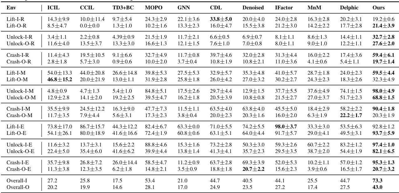
This table presents the average success rate of different offline reinforcement learning algorithms across 18 tasks categorized into three environments (Lift, Unlock, Crash). Each environment has three variations (Random, Medium, Expert) reflecting different data qualities, resulting in 18 tasks. The table shows the mean and 95% confidence interval of the success rates for each algorithm and task, calculated across 10 random seeds. Bold values indicate the best performing algorithm for each task. The p-values are provided to indicate the statistical significance of the differences in performance compared to the best algorithm.
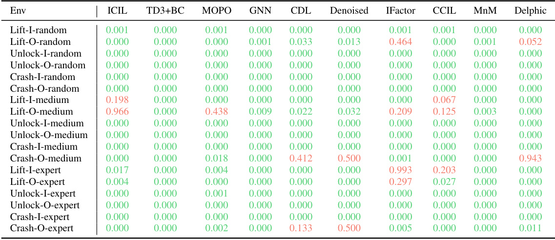
This table presents the statistical significance tests comparing the performance of the proposed BECAUSE method against 10 baseline methods across 18 different tasks. Each task is evaluated using 10 different random seeds, resulting in 180 total comparisons. A p-value is calculated for each comparison, indicating whether the performance of BECAUSE is significantly better than the baseline method. The table visually highlights the significant differences (p<0.05) using color-coding.
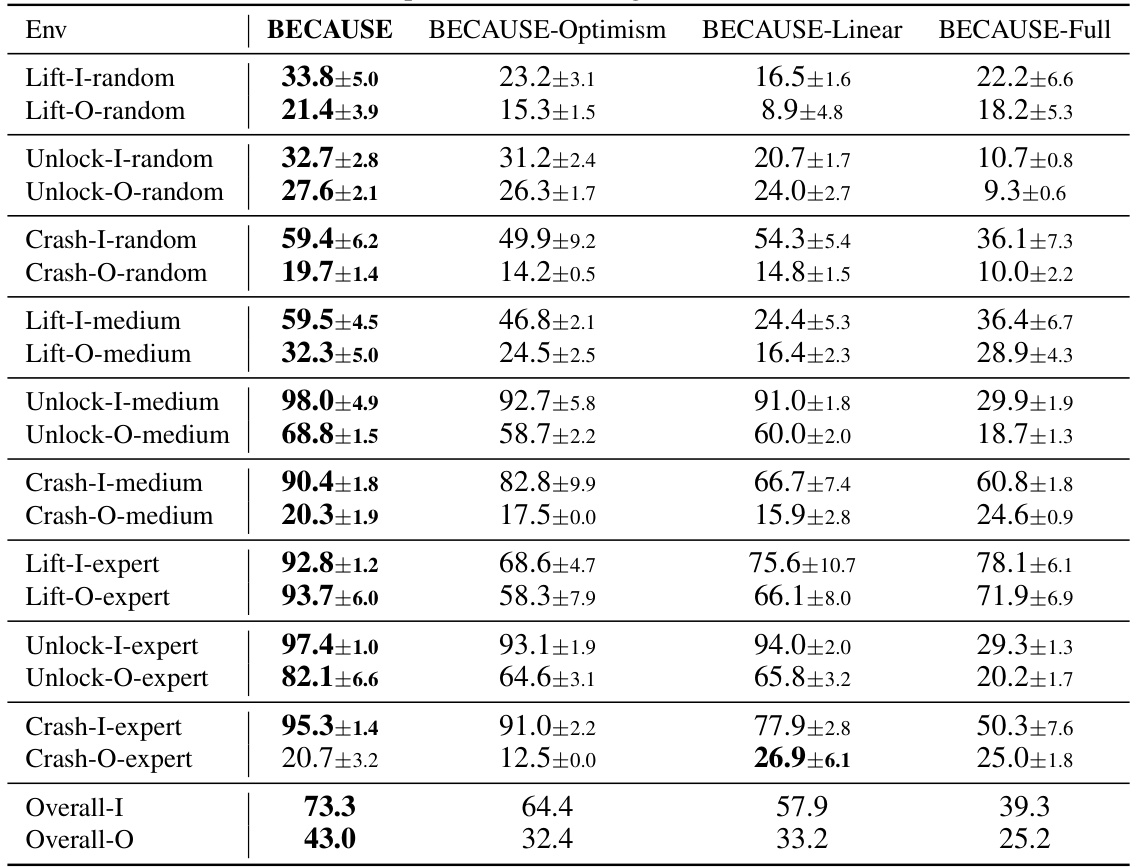
This table presents the average success rates for 18 different reinforcement learning tasks across three environments (Lift, Unlock, Crash), categorized by data quality (random, medium, expert). The results are averaged over 10 trials with 95% confidence intervals and p-values to compare the performance of the BECAUSE algorithm against baselines. Bold values indicate the best-performing algorithm for each task.

This table presents the p-values resulting from statistical significance tests comparing BECAUSE against 10 baseline methods across 18 different tasks. A p-value less than 0.05 indicates a statistically significant difference, with green highlighting indicating that BECAUSE outperformed the baseline. The table demonstrates BECAUSE’s superior performance across a wide range of scenarios.
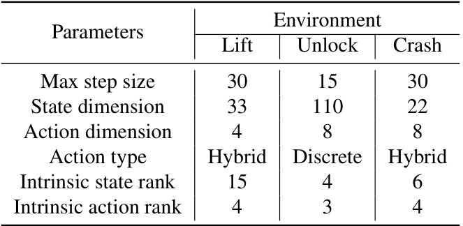
This table summarizes the key parameters and characteristics of the three different reinforcement learning environments (Lift, Unlock, Crash) used in the experiments described in the paper. It shows the maximum number of steps allowed per episode, the dimensionality of the state and action spaces, the type of actions (hybrid, discrete, or hybrid), and the intrinsic rank of the state and action spaces. This information provides context for understanding the complexity and nature of the tasks faced by the reinforcement learning agents.

This table shows the behavior policies used to generate offline datasets for three different environments: Lift, Unlock, and Crash. For each environment, three types of behavior policies were used: Random, Medium, and Expert. The table lists the number of episodes collected for each policy type and the resulting success rate. The ‘Additional Description’ column provides qualitative details on the characteristics of each policy type. This information is crucial for understanding the quality and characteristics of the data used to train the reinforcement learning models in the paper.
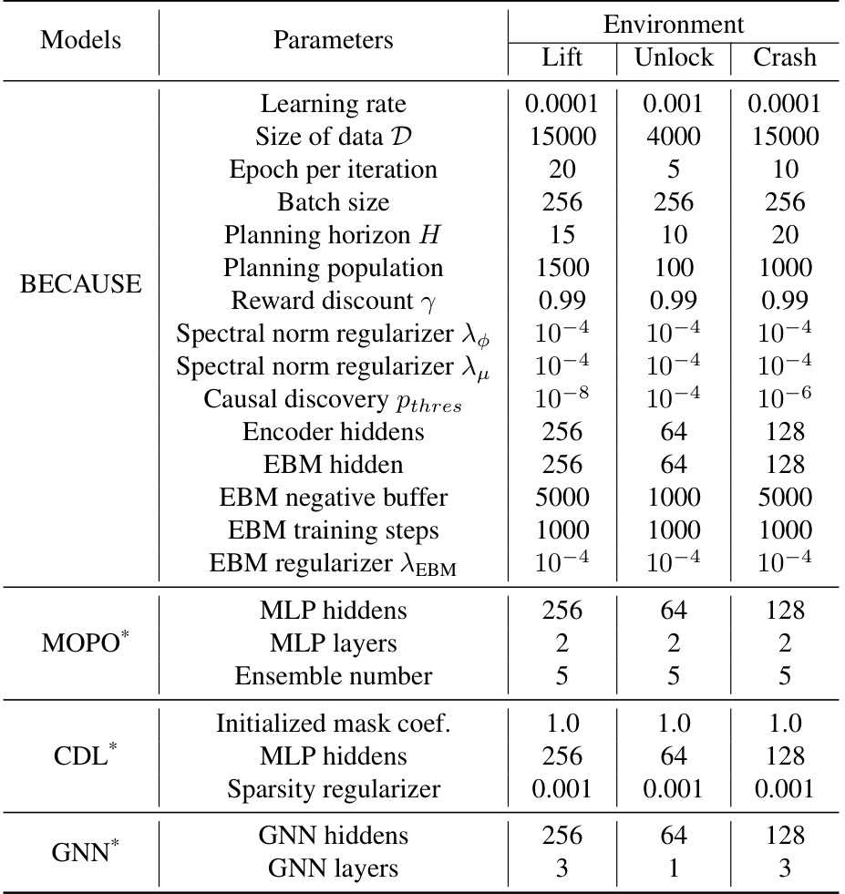
This table lists the hyperparameters used for training the BECAUSE model and several baseline models across three different reinforcement learning environments: Lift, Unlock, and Crash. The hyperparameters are categorized by model (BECAUSE, MOPO, CDL, GNN) and parameter type (learning rate, data size, batch size, planning horizon, reward discount, regularization parameters, network architecture specifics etc.). The table shows that different models required different hyperparameter settings for optimal performance in each environment.
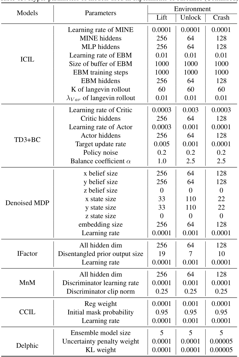
This table lists the hyperparameters used for the BECAUSE model and several baseline models in the experiments described in the paper. It includes parameters related to training, the planning process, and other model-specific settings. The table is divided into sections for each model, making it easy to compare the different configurations used.
Full paper#
