↗ OpenReview ↗ NeurIPS Homepage ↗ Chat
TL;DR#
Teaching machine learning models efficiently is crucial. Traditional methods often require massive datasets, especially when teaching a group of learners with varying characteristics. This paper focuses on a specific type of learner called “Behavior Cloning” that learns by mimicking examples, and specifically explores linear BC learners. The challenge lies in finding the smallest possible dataset to teach a target policy to an entire class of these learners.
This research proposes a new algorithm called ‘TIE’ to solve this problem. TIE cleverly leverages the structure of the problem to construct a minimal teaching set. The paper shows that this problem is computationally hard for complex scenarios, but TIE provides a good approximation with theoretical guarantees. The effectiveness of TIE was demonstrated through experiments in several diverse environments.
Key Takeaways#
Why does it matter?#
This paper is important because it tackles a crucial challenge in machine teaching: efficiently teaching a diverse group of learners. It introduces a novel algorithm with theoretical guarantees, offering a more efficient and effective approach to teaching complex tasks compared to existing methods. This opens new avenues for research into personalized and scalable machine teaching strategies, impacting fields like education and AI.
Visual Insights#

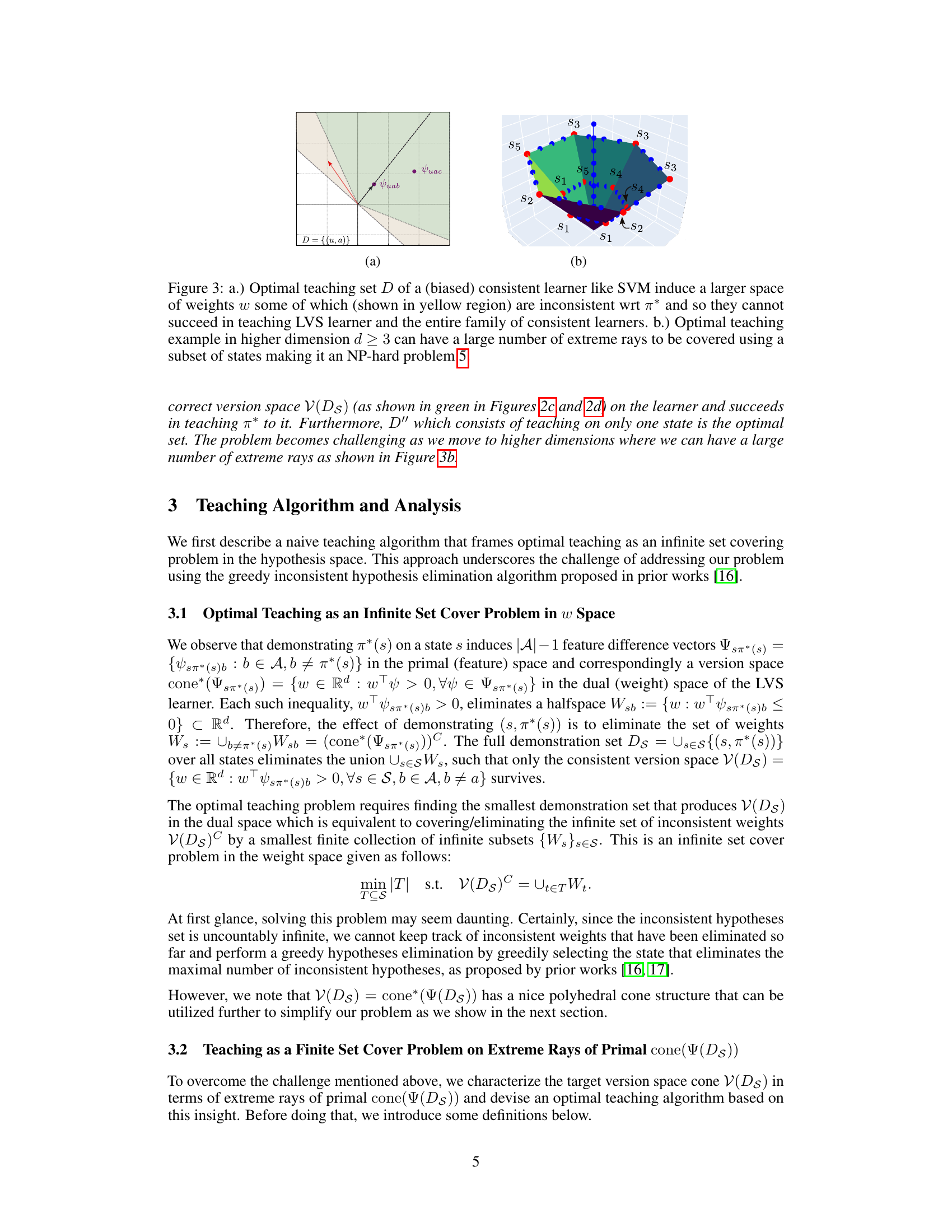
This figure illustrates the concept of extreme rays in the context of teaching a linear version space learner. The version space V(D) is represented by the green shaded area, and the primal cone cone(Ψ(D)) is represented by the blue shaded area. The dots represent feature difference vectors. The figure shows four different datasets (D, D’, D’, D'). While D, D’, and D’ successfully teach the target policy, dataset D fails. This demonstrates that simply covering a sufficient number of feature difference vectors may not guarantee successful teaching. The key lies in covering the extreme rays (edges) of the primal cone.
In-depth insights#
Linear BC Teaching#
The concept of ‘Linear BC Teaching’ presents a fascinating challenge in machine teaching. It focuses on the problem of efficiently teaching a family of linear Behavior Cloning (BC) learners, a common approach in reinforcement learning. The key challenge lies in finding a minimal dataset that can uniquely teach the optimal policy to all learners in the family, despite their potential individual biases and hypothesis preferences. The authors propose a novel algorithm, likely exhibiting an efficient approximation for teaching larger action spaces, addressing the NP-hard nature of the problem for scenarios with more than two actions. This approach highlights the trade-off between teaching the entire family versus optimizing for specific learners, ultimately focusing on achieving a solution that generalizes well across a diverse class of BC algorithms. Understanding the computational complexity and finding effective teaching strategies are essential steps towards building robust machine teaching systems. This research likely contributes valuable insights into optimal teaching strategies for a wide range of BC learners. The findings could have significant implications for real-world applications such as robotics and autonomous driving, where efficient and effective teaching methods are crucial for success.
TIE Algorithm#
The TIE (Teaching Iterative Elimination) algorithm is a novel approach to optimal teaching in the context of a family of linear Behavior Cloning learners. Its core innovation lies in framing the teaching problem as a finite set cover problem over the extreme rays of the primal cone, rather than tackling the more complex infinite set cover problem directly in the hypothesis space. This crucial shift simplifies the computational aspects significantly, allowing for efficient solution finding. TIE proceeds in two stages: first identifying the extreme rays of the primal cone using an iterative linear programming approach, and then solving the finite set cover problem to find a minimal subset of states that cover these rays. The algorithm’s efficiency is particularly noteworthy, especially when the action space is small (|A| ≤ 2), where it achieves instance optimality in teaching dimension. However, for larger action spaces, the set cover problem becomes NP-hard, though TIE offers an efficient approximation algorithm with a logarithmic approximation ratio (log(|A| -1)), demonstrating its practicality even in complex scenarios. Overall, TIE presents a significant advance in machine teaching, offering a computationally feasible and theoretically grounded solution for teaching a family of linear BC learners.
NP-hardness Proof#
The NP-hardness proof section would rigorously demonstrate that optimally teaching a family of linear behavior cloning learners is computationally intractable for action spaces larger than two. This would likely involve a reduction from a known NP-complete problem, such as Set Cover, to the optimal teaching problem. The proof would construct a polynomial-time transformation mapping instances of the NP-complete problem to instances of the optimal teaching problem, showing that a solution to the teaching problem efficiently solves the NP-complete problem. Crucially, the reduction would showcase how the complexity of the optimal teaching problem scales exponentially with the size of the action space when |A| > 2, highlighting the inherent difficulty of finding the absolute smallest dataset for teaching. This proof would formally establish a fundamental limitation of achieving optimal teaching for this class of learners in complex scenarios, justifying the need for approximation algorithms as presented in the paper.
Empirical Results#
A strong ‘Empirical Results’ section would go beyond simply presenting numbers; it would weave a compelling narrative. It should begin by clearly stating the goals of the experiments: what hypotheses are being tested and what questions are being answered. Then, the results should be presented concisely but completely, perhaps using tables or figures to highlight key findings. Crucially, the discussion of results should not just describe what was found, but also interpret those findings. Comparisons to baselines are essential to show the method’s improvement. Finally, limitations of the experiments should be acknowledged, and future research directions suggested. Statistical significance, where appropriate, is vital for establishing the reliability of findings, and error bars on graphs provide a crucial visual cue. The overall impression should be one of rigor, transparency, and insightful analysis, not just data presentation. The writing should be clear and engaging, guiding the reader through the evidence and its implications.
Future Work#
The paper’s ‘Future Work’ section suggests several promising avenues. Extending the optimal teaching framework beyond deterministic policies to encompass stochastic policies would significantly broaden its applicability. Similarly, scaling the approach to handle non-linear learners is crucial for tackling real-world complexities. The current assumption of a fully-informed teacher who can freely access and demonstrate any state might be unrealistic. Investigating teaching under budget constraints, where the teacher’s actions are limited, would make the model more practical. Exploring how to efficiently navigate complex state spaces and strategically select demonstrations when the teacher’s interaction is costly is a critical direction. Finally, considering scenarios with multiple, potentially conflicting, learners is a relevant area for future exploration, potentially revealing methods to balance individual learner needs within a group setting.
More visual insights#
More on figures
This figure demonstrates the importance of covering extreme rays of the primal cone in the optimal teaching problem for linear behavior cloning learners. It shows four datasets (D, D’, D’, and D’’’) and their corresponding primal cones and version spaces. Datasets D, D’, and D’ successfully teach the target policy, while dataset D fails because it does not cover all the extreme rays of the primal cone. This illustrates that a teaching set must cover all the extreme rays to unambiguously teach the entire family of consistent linear BC learners.

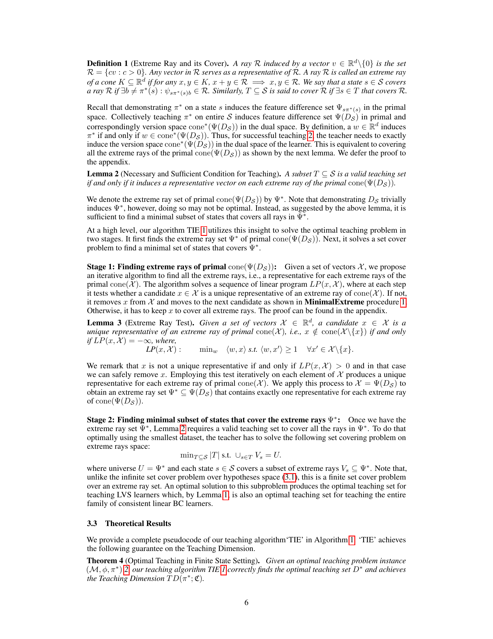
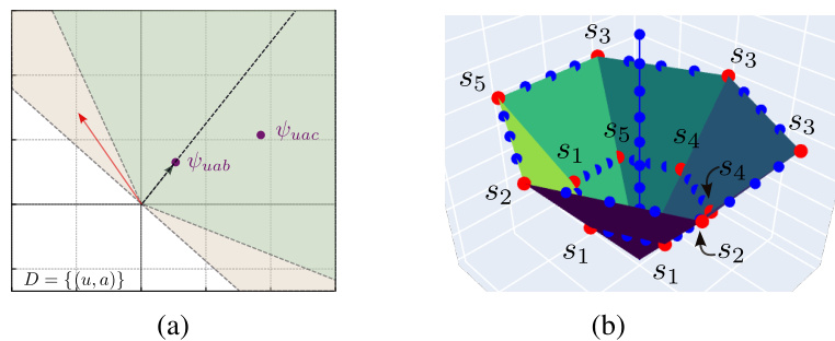
This figure demonstrates the results of the optimal teaching algorithm Greedy-TIE on the ‘Pick the Right Diamond’ game with 6 slots. Panel (a) shows a visualization of the feature space, highlighting the primal cone, dual version space, and the feature difference vectors. Panel (b) displays a teaching set generated by Greedy-TIE. Panel (c) presents a comparison of Greedy-TIE’s performance against other baselines (Teach-All and Teach-Random) in terms of teaching set size, demonstrating Greedy-TIE’s superior efficiency in reducing the dataset required for effective teaching.

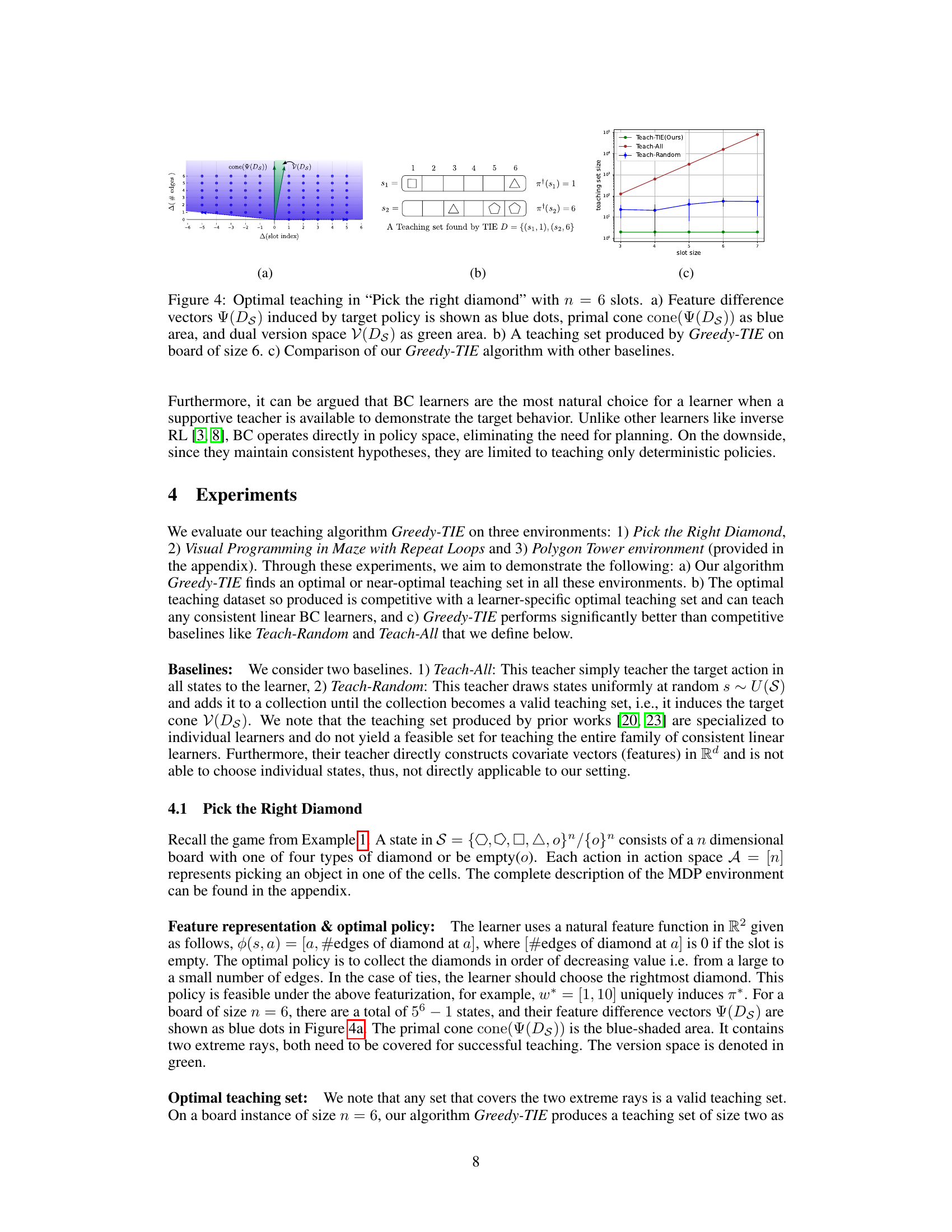
Figure 5(a) shows an example of a visual programming task in a 5x5 maze. The goal is to programmatically guide a turtle to a goal location using a limited set of code blocks (move forward, turn left, turn right, repeat). Figure 5(b) presents a graph comparing the performance of the proposed Greedy-TIE algorithm against two baseline approaches (Teach-All and Teach-Random) across mazes of varying sizes. The y-axis represents the size of the teaching set, while the x-axis shows the grid size of the maze.

This figure shows the optimal teaching set generated by the Greedy-TIE algorithm for a goal-reaching coding task on a 5x5 maze. The teaching set consists of a sequence of states, each showing the initial board (without any partial code) and the optimal action (code block) to take in that state. The figure demonstrates how the algorithm produces a compact and efficient set of demonstrations that is sufficient to teach the target policy to the entire family of consistent linear BC learners.
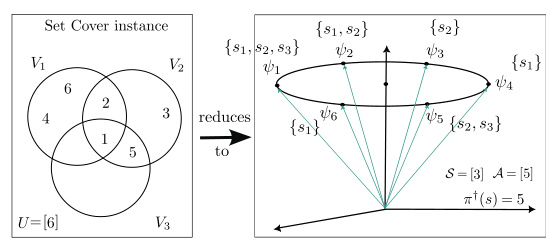
This figure demonstrates a reduction from a set cover problem to an optimal teaching linear behavior cloning (LBC) problem. It shows how a set cover instance (left side) with a universe U and subsets V1, V2, and V3 can be mapped to an equivalent optimal teaching instance (right side) with states S corresponding to the subsets and actions A related to the size of the universe and the target policy. The mapping ensures that a solution to the set cover problem directly translates to a solution to the teaching problem and vice versa, proving the NP-hardness of the optimal teaching problem.

This figure visualizes the results of the Polygon Tower experiment. Subfigure (a) shows all feature difference vectors for n=6, illustrating the data used in the experiment. Subfigure (b) provides a top-down view of the extreme vectors in the primal cone when n=6, highlighting the key features for optimal teaching. Subfigure (c) presents a graph showing the running time of the TIE algorithm against the increasing size of the problem (n). Finally, subfigure (d) compares the optimal teaching dimension to the teaching set size obtained by TIE, demonstrating that TIE accurately finds the optimal teaching set in this scenario.
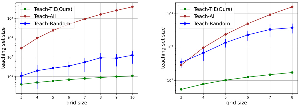
The figure compares the performance of three teaching algorithms: Teach-TIE (the proposed algorithm), Teach-All (teaching all states), and Teach-Random (randomly selecting states until a valid teaching set is obtained). The comparison is shown for two different feature representations: local features (left panel) and global features (right panel). The x-axis represents the grid size of the maze in the visual programming task, and the y-axis shows the size of the teaching set generated by each algorithm. Error bars are included to indicate the variability in the results. The results suggest that Teach-TIE consistently requires a smaller teaching set size compared to the other baselines, demonstrating its efficiency in teaching the visual programming task.
Full paper#
