↗ OpenReview ↗ NeurIPS Homepage ↗ Chat
TL;DR#
Training recurrent neural networks (RNNs) efficiently in online reinforcement learning is challenging due to the computational cost of standard methods like Real-Time Recurrent Learning (RTRL). Existing approaches either approximate RTRL, leading to biased gradient estimates, or restrict RNN architectures, limiting representational power. This paper tackles these issues.
This work introduces Recurrent Trace Units (RTUs), a lightweight modification to Linear Recurrent Units (LRUs). RTUs leverage complex-valued diagonal recurrences, making RTRL efficient. Experiments across several partially observable environments show that RTUs significantly outperform existing RNN architectures in terms of performance and computational efficiency when trained with RTRL. The findings are particularly relevant to online reinforcement learning where agents learn and interact with their environments simultaneously.
Key Takeaways#
Why does it matter?#
This paper is important because it presents a novel and efficient method for training recurrent neural networks (RNNs) in online reinforcement learning, a significant challenge in the field. The proposed approach, using Recurrent Trace Units (RTUs), offers substantial performance gains over existing methods while requiring significantly less computation. This opens avenues for deploying RNNs in real-world applications where real-time learning is crucial and computational resources are limited, pushing the boundaries of online RL.
Visual Insights#

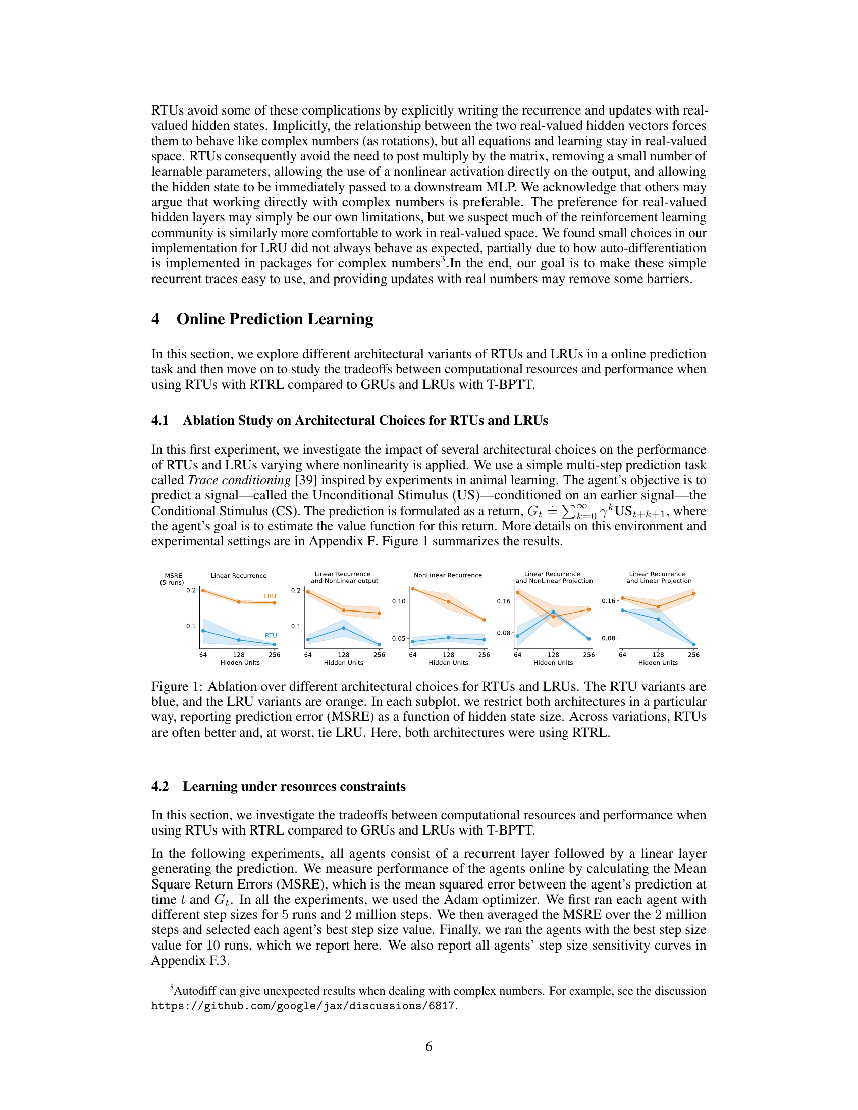
This figure shows the ablation study on architectural choices for Recurrent Trace Units (RTUs) and Linear Recurrent Units (LRUs). Different architectural variations are tested, including linear recurrence, linear recurrence with nonlinear output, nonlinear recurrence, linear recurrence with nonlinear projection, and linear recurrence with linear projection. The Mean Squared Return Error (MSRE) is plotted against the number of hidden units for each architecture. The results demonstrate that RTUs generally outperform or match the performance of LRUs across different architectural choices, especially when employing Real-Time Recurrent Learning (RTRL).
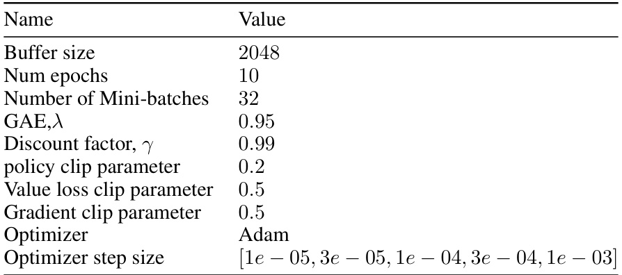
This table lists the hyperparameters used for the Proximal Policy Optimization (PPO) algorithm in the paper’s experiments. It includes settings for buffer size, number of epochs, minibatch size, Generalized Advantage Estimation (GAE) lambda, discount factor, policy and value loss clipping parameters, optimizer (Adam), and a range of optimizer step sizes explored.
In-depth insights#
RTUs: A Deep Dive#
A hypothetical section titled “RTUs: A Deep Dive” in a research paper would likely offer a detailed technical exploration of Recurrent Trace Units. It would begin by formally defining RTUs, contrasting them with related architectures like LRUs (Linear Recurrent Units) and GRUs (Gated Recurrent Units), highlighting their unique features such as the use of complex-valued diagonal recurrence and the incorporation of non-linearity. The core of this section would delve into the mathematical underpinnings of RTUs, including a thorough derivation of their RTRL (Real-Time Recurrent Learning) update rules and a comprehensive analysis of their computational complexity. The authors would likely present empirical evidence demonstrating the benefits of RTUs, including comparisons with alternative architectures in terms of prediction accuracy, sample efficiency, and computational cost, using various benchmark environments. Further investigation might include ablation studies showing the impact of design choices like the type of non-linearity and its position within the RTU structure. Finally, the “deep dive” would discuss any limitations or potential challenges associated with RTUs and outline directions for future research. A key focus would be on showing how the seemingly small modifications to LRUs in RTUs result in substantial improvements in practical performance for online reinforcement learning settings.
RTRL Efficiency#
Real-Time Recurrent Learning (RTRL) offers a theoretically appealing approach to training recurrent neural networks (RNNs) by directly calculating the gradient during online learning, thus avoiding the limitations of truncated backpropagation through time (TBPTT). However, standard RTRL suffers from a quartic time complexity, making it computationally prohibitive for large networks. The core challenge addressed in many papers is how to achieve the benefits of RTRL’s exact gradient without the massive computational burden. Approaches often involve restricting the RNN architecture to simpler forms, such as linear or diagonal recurrent layers, which allow for more efficient RTRL implementation. This often comes at the cost of reduced representational capacity. Researchers explore various strategies to improve RTRL efficiency, including using complex-valued diagonal recurrence to maintain representational power while simplifying computations. This involves representing the recurrent weights with complex numbers, leveraging a mathematical equivalence to reduce the computational cost associated with the RTRL update. The effectiveness of these techniques hinges on finding architectural modifications that balance computational efficiency with the capacity to learn complex temporal dependencies. The pursuit of RTRL efficiency remains a critical area of research for online RNN training, with the goal of bridging the gap between the theoretical appeal and practical feasibility of RTRL for real-world applications.
Online RL#
Online reinforcement learning (RL) presents unique challenges and opportunities compared to offline RL. The core challenge lies in the agent’s need to learn and adapt continuously while interacting with an environment, without the benefit of pre-collected datasets for training. This necessitates algorithms capable of efficient online learning, such as Real-Time Recurrent Learning (RTRL), which can update model parameters after each interaction without needing to store past experiences. However, RTRL’s high computational cost has limited its use in practical applications. This research explores ways to address this computational burden via lightweight recurrent architectures, particularly Recurrent Trace Units (RTUs). The focus is on creating efficient learning methods suitable for partially observable environments, which are characterized by incomplete or noisy sensory information. This requires robust state representation mechanisms which can successfully summarize past information within constrained computational budgets, making the approach suitable for real-world scenarios. The animal-learning prediction task and various Mujoco control experiments demonstrate RTU’s effectiveness. This work highlights the trade-off between computational efficiency and model capacity, showcasing that RTUs strike a favorable balance in online RL scenarios while outperforming conventional methods in environments requiring strong temporal processing capabilities.
Architectural Choices#
The section on “Architectural Choices” would delve into the design decisions behind the recurrent neural network (RNN) architecture employed in the research. It would likely compare different RNN variants, such as Recurrent Trace Units (RTUs), Gated Recurrent Units (GRUs), and Linear Recurrent Units (LRUs), analyzing their strengths and weaknesses in the context of real-time reinforcement learning (RL). A key aspect would be evaluating the trade-offs between computational efficiency and representational power. The analysis would likely highlight how the choice of architecture impacts the feasibility of using Real-Time Recurrent Learning (RTRL), a computationally expensive but exact gradient calculation method preferred for online RL scenarios. The discussion could also involve an analysis of how different parameterizations and non-linearities within the chosen architectures affect learning performance and stability, possibly focusing on the use of complex-valued weights in some architectures. Ultimately, the section aims to justify the selection of a specific RNN architecture (likely RTUs) based on its overall effectiveness in the studied partially-observable RL environments. Emphasis would be placed on demonstrating how the chosen architecture enables efficient training using RTRL while maintaining strong performance.
Future Work#
The paper’s lack of a dedicated ‘Future Work’ section is notable. However, we can infer potential future research directions based on the limitations and open questions raised. Extending RTUs to handle multilayer recurrent networks is a significant challenge requiring a more principled approach for tracing gradients across layers. The current approach of treating each layer independently sacrifices the potential benefits of true multi-layer recurrence. Further research is needed to address the inherent computational limitations of RTRL. Exploring parallel scan training techniques for RTUs, particularly for non-linear activations, could significantly enhance their scalability and efficiency for larger-scale problems. While RTUs demonstrate significant potential in partially observable environments, further empirical evaluation across a broader set of benchmarks and tasks is necessary to fully assess their generalization capabilities. Additionally, a theoretical analysis comparing RTUs to transformers in online reinforcement learning settings would be valuable to clarify their relative strengths and weaknesses. Finally, investigating the interaction between RTRL and the staleness of gradients in policy gradient methods (such as PPO) warrants further study. Understanding how this staleness affects convergence and overall performance is crucial for optimizing the practical use of RTUs in RL.
More visual insights#
More on figures

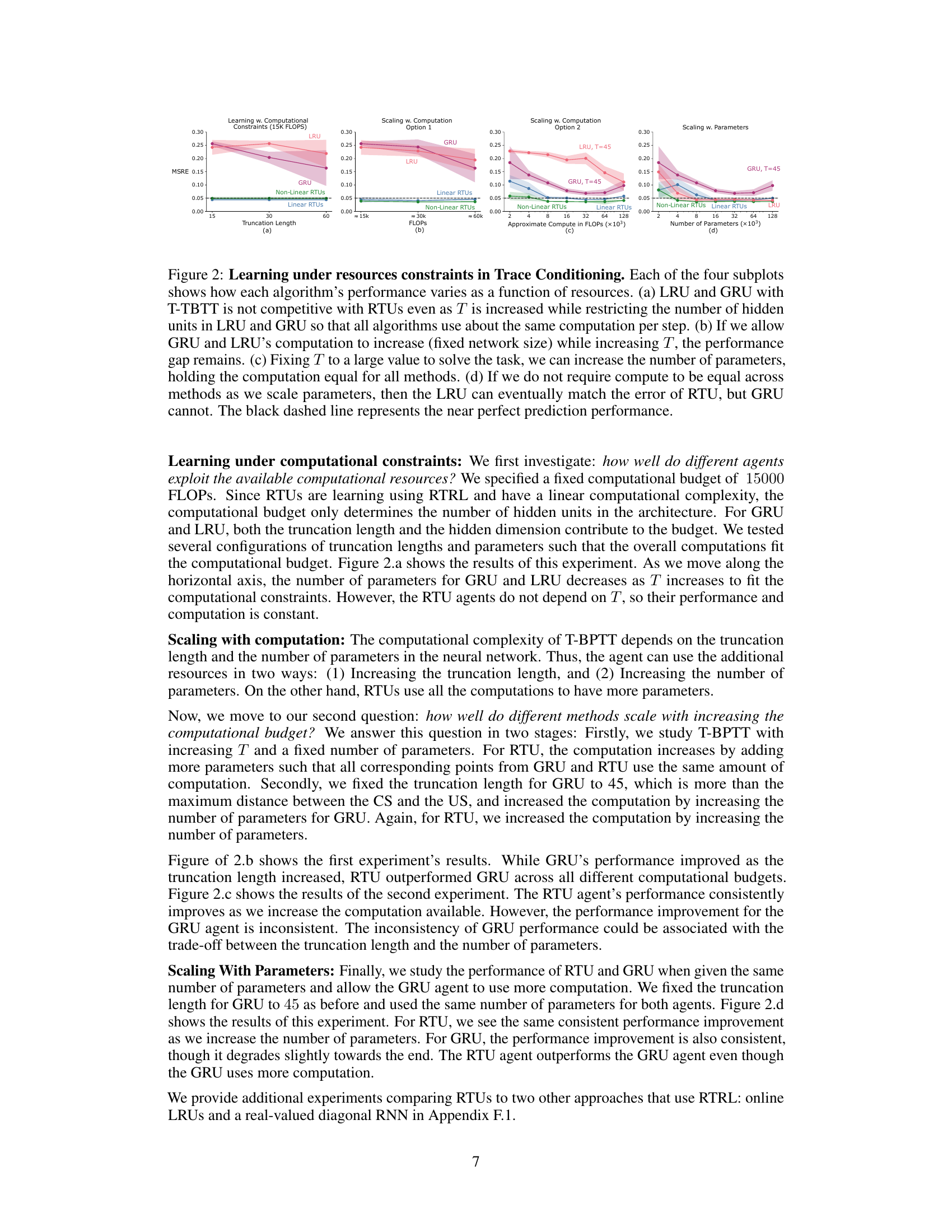
This figure shows the performance of different recurrent neural network architectures (RTUs, LRUs, GRUs) under different computational constraints in a trace conditioning task. Four subplots illustrate how performance changes with increasing computational resources (measured in FLOPs and number of parameters) and truncation length (for GRUs and LRUs). RTUs consistently perform well across different resource levels, highlighting their efficiency.
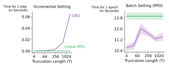
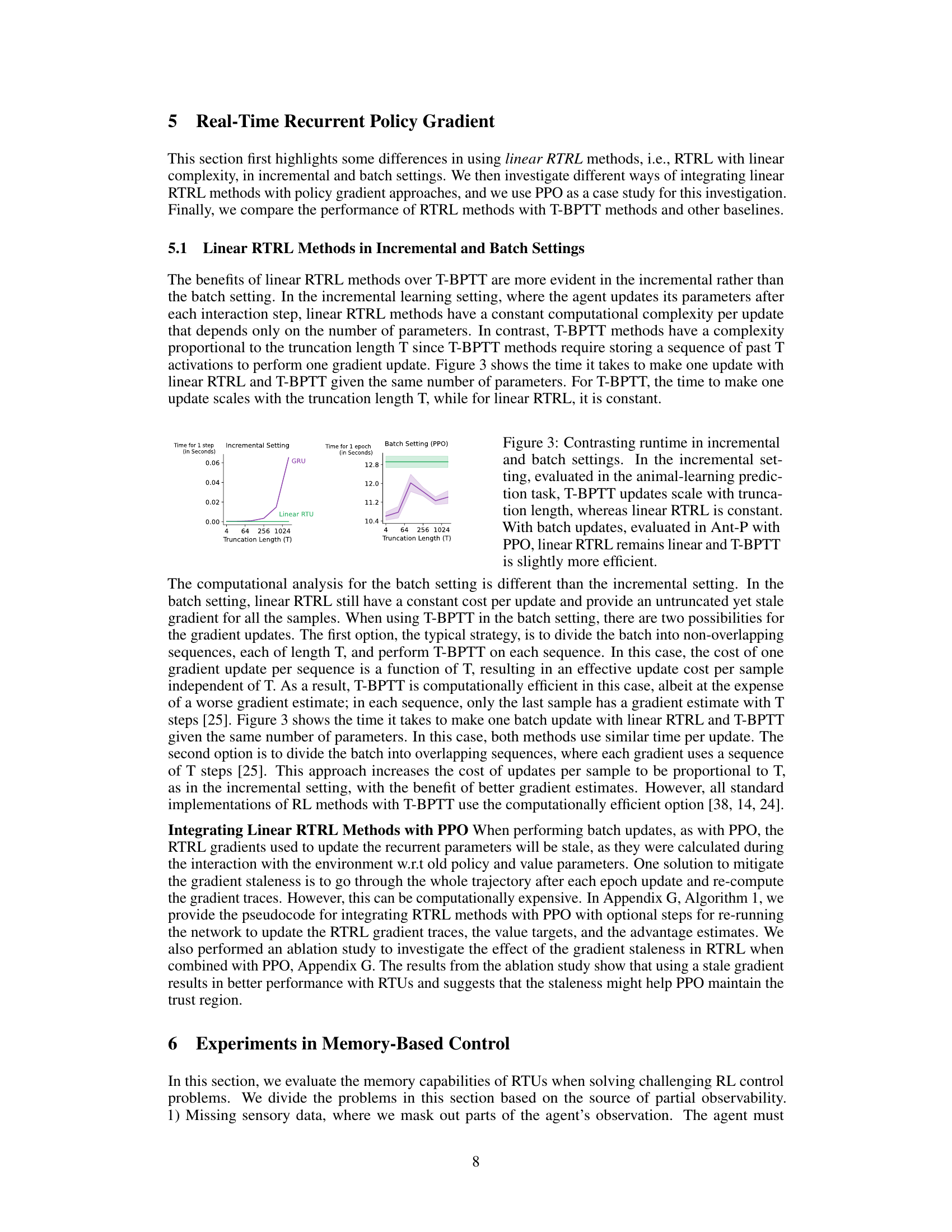
This figure compares the runtime of linear RTRL and T-BPTT methods for incremental and batch settings. The left panel shows that in incremental learning (animal learning prediction task), T-BPTT’s runtime scales linearly with the truncation length (T), while linear RTRL remains constant. The right panel demonstrates that in the batch setting (PPO on the Ant-P environment), linear RTRL maintains its linear runtime, whereas T-BPTT shows more variability but remains relatively efficient, showcasing the advantages of linear RTRL in incremental learning scenarios.
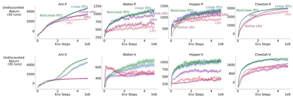
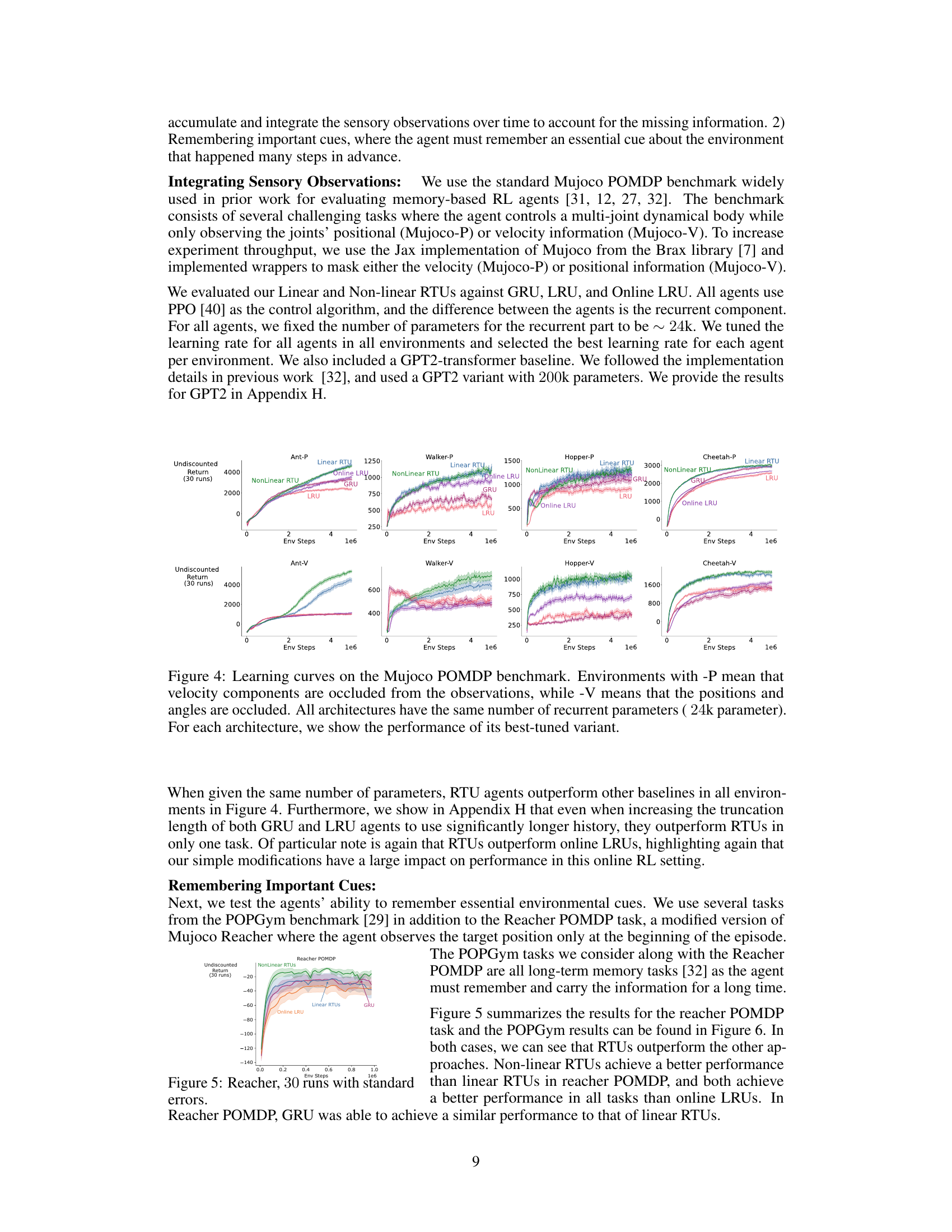
This figure presents the learning curves for different recurrent neural network architectures on the Mujoco Partially Observable Markov Decision Process (POMDP) benchmark. The benchmark consists of several control tasks where the agent’s observations are partially occluded, either by removing velocity information (-P) or by removing position and angle information (-V). The figure shows how well each architecture learns the task over time, as measured by the undiscounted return. All architectures are constrained to use the same number of recurrent parameters (24,000), and the plot shows the results for the best hyperparameter setting for each architecture.

This figure shows the learning curves for different recurrent network architectures on the Reacher POMDP task, which requires remembering important cues over a long time horizon. Non-linear RTUs significantly outperform linear RTUs, online LRUs, and GRUs, demonstrating their ability to effectively utilize information from the past for better performance in this long-term memory task.

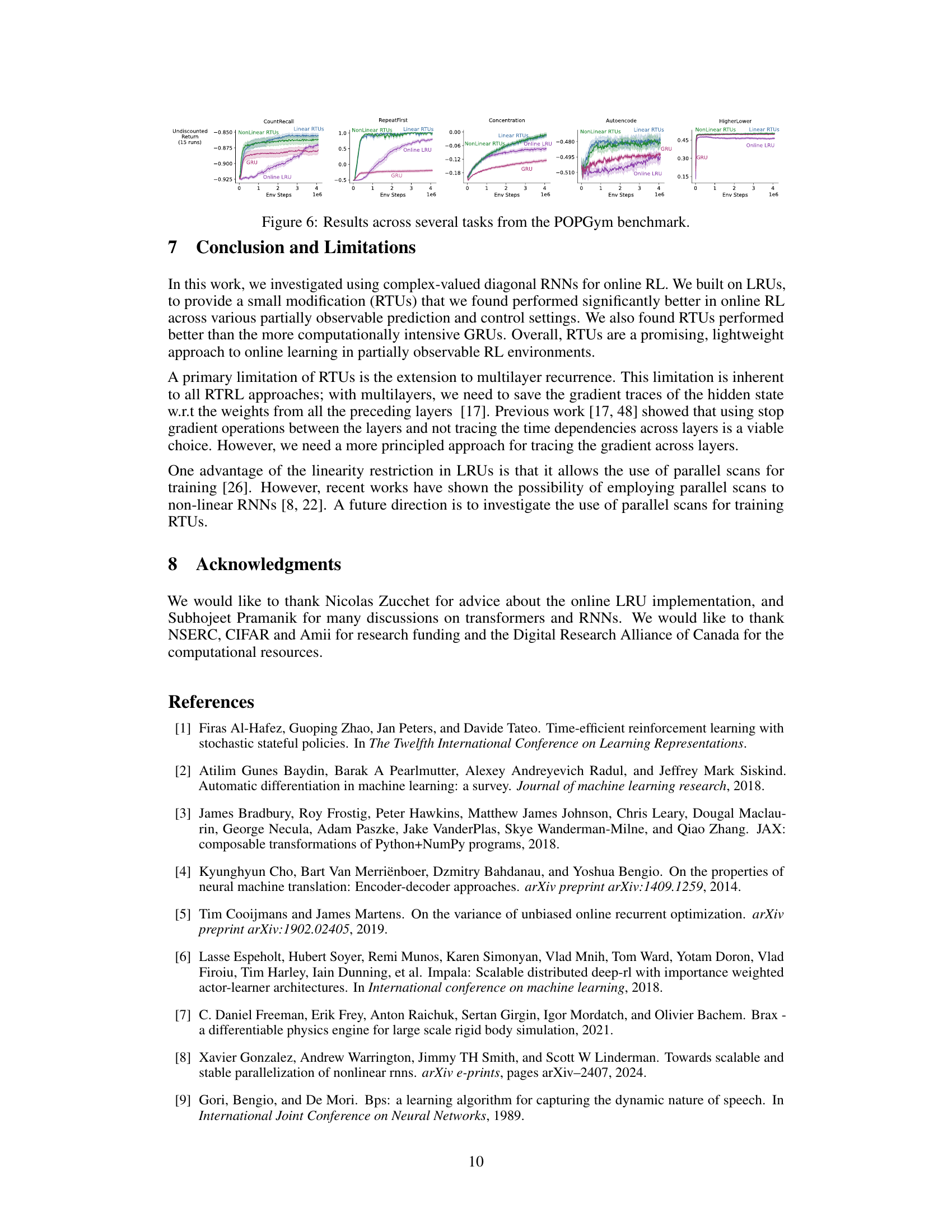
This figure presents the results of multiple experiments conducted on various tasks from the POPGym benchmark. The benchmark likely tests the agents’ ability to handle long-term dependencies and partial observability. Each subplot represents a different task (CountRecall, RepeatFirst, Concentration, Autoencode, HigherLower), showing the undiscounted return achieved by different agents (NonLinear RTUs, Linear RTUs, Online LRU, GRU) over time. The figure demonstrates the comparative performance of different recurrent neural network architectures in tasks requiring memory and decision-making under uncertainty.
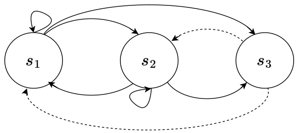
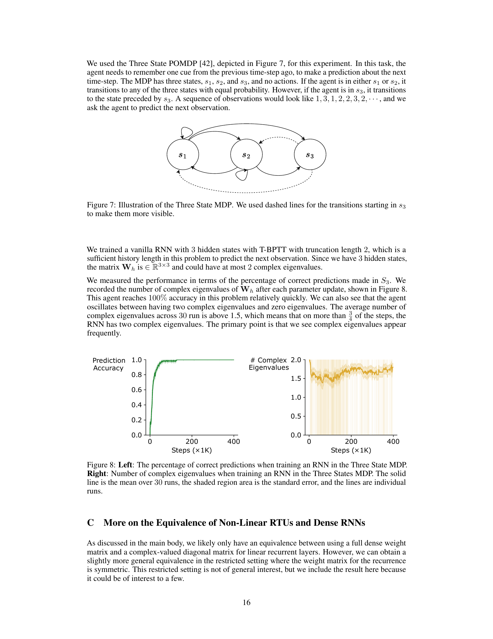
This figure is a state transition diagram for a three-state Markov Decision Process (MDP). The states are represented as circles labeled s1, s2, and s3. Solid lines indicate transitions with equal probability (1/3) from s1 and s2 to each of the three states. The dashed lines represent transitions from s3. From s3, the transitions go deterministically back to the previous state in the sequence, creating a kind of short-term memory effect in the MDP. The self-loops from s1 and s2 indicate that there’s also a probability of staying in the same state.

This figure shows the training process of a vanilla RNN on a three-state POMDP task. The left panel displays the prediction accuracy over training steps, reaching 100%. The right panel shows the number of complex eigenvalues in the weight matrix of the RNN during training, averaging above 1.5 which suggests the frequent appearance of complex eigenvalues during training.
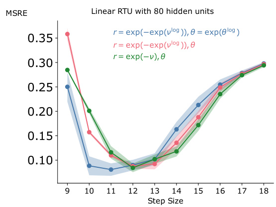
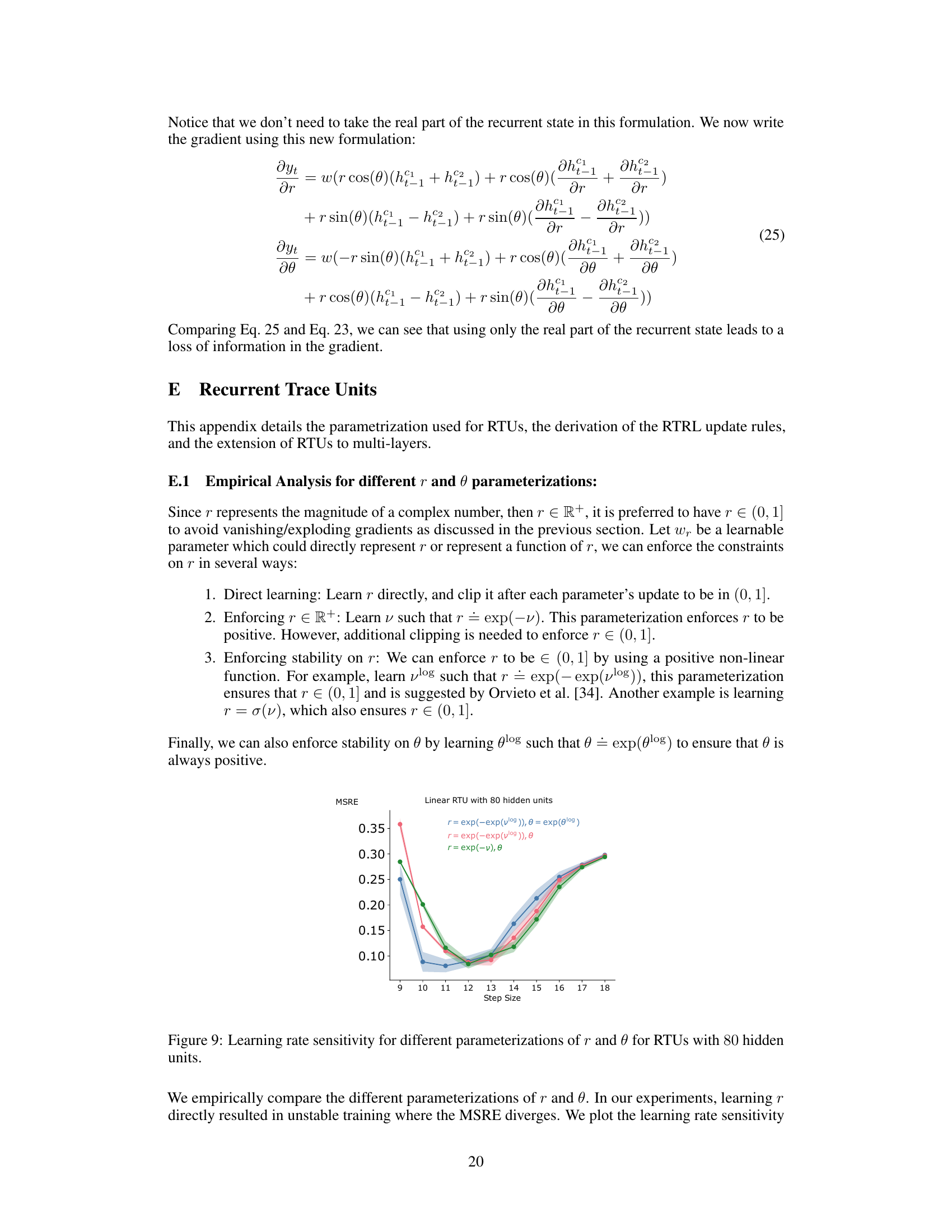
This figure shows the impact of different parameterizations of r and θ on the learning rate sensitivity of RTUs with 80 hidden units. Three different parameterizations are compared: r = exp(-exp(vlog)), θ = exp(θlog); r = exp(-exp(vlog)), θ; and r = exp(-ν), θ. The y-axis represents the Mean Squared Return Error (MSRE), a measure of prediction accuracy. The x-axis represents the step size used during training. The figure shows that different parameterizations lead to different levels of sensitivity to the learning rate, highlighting the importance of careful parameterization in achieving optimal performance.
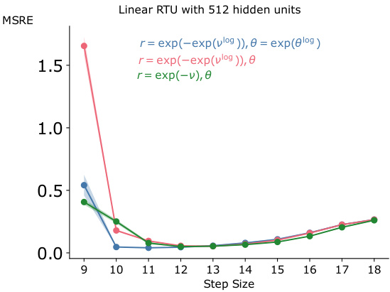
The figure shows the mean squared return error (MSRE) for different learning rates when training a recurrent trace unit (RTU) network with 80 hidden units. Three different parameterizations of the complex-valued diagonal recurrence weights (r and θ) are compared: 1. r = exp(-exp(vlog)), θ = exp(θlog) 2. r = exp(-exp(vlog)), θ 3. r = exp(-v), θ The plot illustrates the impact of different parameterizations on learning stability and optimal learning rate selection. The x-axis shows the learning rate while the y-axis represents the MSRE.
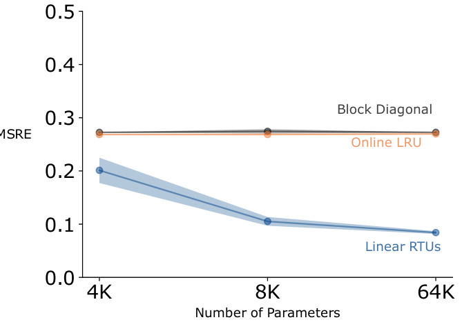
This figure compares the performance of RTUs to other RTRL-based approaches with similar architectures: an online version of LRU and a vanilla block diagonal RNN. The results indicate that seemingly small differences between the diagonal RNNs can result in significantly different behavior. RTUs outperform both online LRUs and block diagonal RNNs. The better performance of RTUs highlights the benefits of using the proposed parameterization and incorporating nonlinearities in the recurrence for achieving better performance in online RL.
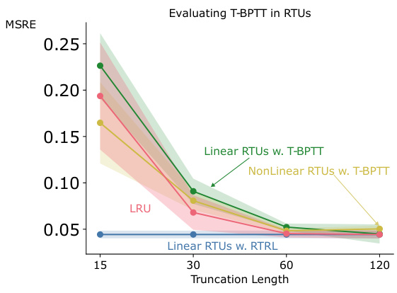
This figure shows the performance comparison between RTUs trained with RTRL and RTUs trained with T-BPTT in the trace conditioning task. The x-axis represents different truncation lengths used for T-BPTT, and the y-axis represents the mean squared return error (MSRE). The results demonstrate that the performance of RTUs trained with T-BPTT approaches that of RTUs trained with RTRL as the truncation length increases, suggesting that using a longer history improves accuracy with T-BPTT.

This figure displays a comprehensive analysis of how different recurrent neural network architectures (RTUs, LRUs, GRUs) perform under varying computational resource constraints in a trace conditioning task. It shows the trade-off between computational budget (measured in FLOPS), truncation length (for T-BPTT algorithms), and the number of parameters. The results demonstrate RTUs’ superior performance and scalability compared to LRUs and GRUs, particularly when computational resources are limited.

This figure shows an ablation study on the performance of different recurrent neural network architectures (RTUs, LRUs, and GRUs) under different computational constraints in a trace conditioning task. It demonstrates that RTUs consistently outperform LRUs and GRUs, particularly when computational resources are limited. The figure also illustrates how performance varies when resources are allocated to increasing either truncation length or the number of parameters.

This figure presents an ablation study comparing different architectural variants of RTUs and LRUs on a multi-step prediction task. Five different architectural variations are tested for both RTUs and LRUs, focusing on where non-linearity is applied in the network. The mean squared return error (MSRE) is reported for different sizes of the hidden state, demonstrating the impact of architectural choices on prediction accuracy. RTUs consistently perform as well as, or better than, LRUs across all variations. Note that all models used RTRL in this experiment.

This figure displays the learning rate sensitivity curves for linear and nonlinear RTUs with various hidden unit counts (160, 800, 450, 230, 6100, 3200, 1650) in the animal learning benchmark. The plots show how the mean squared return error (MSRE) changes with different learning rates, providing insights into the optimal learning rate range for RTUs of various sizes and types.

This figure shows the learning rate sensitivity curves for linear and non-linear RTUs in the animal learning prediction benchmark. It displays how the mean squared return error (MSRE), a measure of prediction accuracy, changes with different learning rates and varying numbers of hidden units (h) within the RTUs. The different colors and shades represent different numbers of hidden units. The graph helps to identify the optimal learning rate range for each RTU configuration to achieve the best prediction performance.

This figure shows the results of an ablation study investigating the effects of stale gradients and stale targets when using RTRL with PPO on the Ant environment from the Mujoco POMDP benchmark. The experiment compares four conditions: (1) both the gradient and target are computed using the latest data; (2) the gradient is stale but the target is fresh; (3) the gradient is fresh but the target is stale; and (4) both the gradient and target are stale. The results indicate that using stale gradients leads to better performance than using fresh gradients, and suggest that stale gradients might help PPO maintain the trust region. A rightmost subplot shows the approximate KL divergence between the two policies, illustrating how agents with stale gradients move away from the old policy more slowly than agents with fresh gradients, possibly suggesting that stale gradients might help with maintaining the trust region.
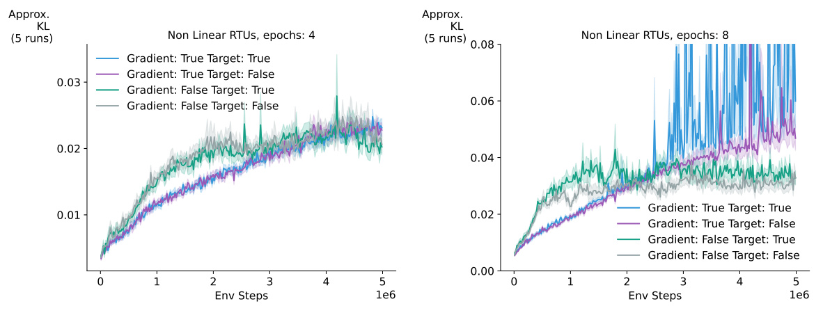
This figure shows an ablation study on the effects of stale gradients and stale targets when using RTUs with PPO on the Ant environment. It compares four scenarios: using true gradients and true targets, true gradients and false targets, false gradients and true targets, and false gradients and false targets. The results indicate that using stale gradients leads to better performance compared to recomputing the gradient, suggesting that stale gradients may help PPO maintain the trust region. The impact of stale value targets and advantage estimates is minimal.
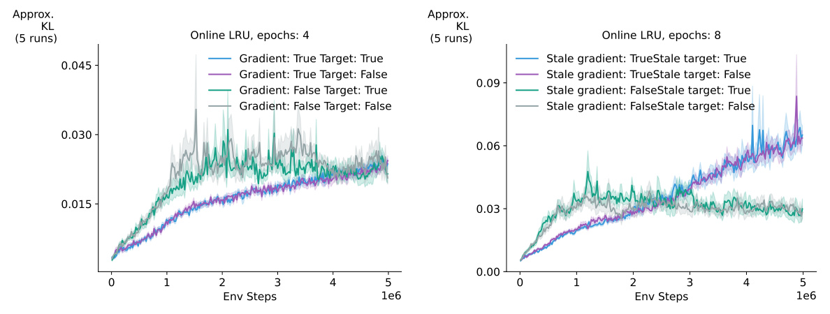
This figure shows an ablation study on the effects of stale gradients and targets when using RTRL with PPO on the Ant environment. It compares four scenarios: using fresh gradients and targets, using fresh gradients with stale targets, using stale gradients with fresh targets, and using stale gradients and stale targets. The results show that using stale gradients consistently leads to better performance than recomputing the gradients, regardless of whether the targets are stale or fresh. This suggests a possible benefit from using stale gradients in this specific setting.
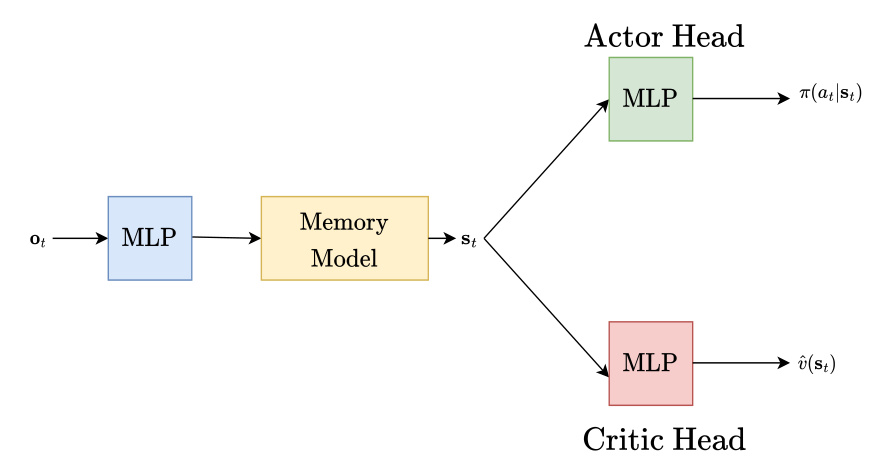
This figure shows the architecture of the agents used in the control experiments. The observation is first passed through an MLP, which then feeds into a memory model (either a Recurrent Trace Unit (RTU), Linear Recurrent Unit (LRU), or Gated Recurrent Unit (GRU)). The output of the memory model is then passed to two separate MLPs: one for the actor head that outputs the action, and one for the critic head that outputs the state value.

This figure displays the learning curves for several different reinforcement learning agents on a set of MuJoCo environments. The environments are partially observable, meaning some information about the state of the environment is hidden from the agent. The ‘P’ versions of the environments hide velocity information, while the ‘V’ versions hide position and angle information. Each line represents a different RL algorithm (NonLinear RTU, Linear RTU, GRU, Online LRU, LRU) which are each attempting to learn an optimal control policy for their respective environments. The x-axis represents training steps, and the y-axis represents the total discounted reward. All algorithms used the same number of parameters, allowing for a comparison based on architectural differences rather than simply computational resources.

This figure displays the learning curves for different recurrent neural network architectures (NonLinear RTU, Linear RTU, GRU, Online LRU, and LRU) on various Mujoco POMDP benchmark tasks. The benchmark tasks involve partially observable environments where either velocity or positional information is hidden. The results show the undiscounted return over the course of 1 million environment steps. All architectures are constrained to have the same number of recurrent parameters. The best performing variant of each architecture is presented in the plot.

This figure compares the performance of RTUs, GRUs, and LRUs under various resource constraints in the Trace Conditioning task. It demonstrates that RTUs outperform other methods across different resource settings. Subplots show performance changes with varying truncation length (T), compute (FLOPS), and number of parameters.

This figure presents an ablation study comparing the performance of Recurrent Trace Units (RTUs) and Linear Recurrent Units (LRUs) across different architectural variations. Each subplot shows a comparison with a specific architectural constraint (e.g., linear recurrence with nonlinear output, nonlinear recurrence), showing mean squared return error (MSRE) plotted against the number of hidden units. The results indicate that RTUs generally outperform or match the performance of LRUs across various architectures when both use the Real-Time Recurrent Learning (RTRL) algorithm.

This figure presents an ablation study comparing the performance of RTUs, GRUs, and LRUs under different resource constraints in a trace conditioning task. Subplots (a), (b), and (c) show how performance varies with different levels of computational budget, while subplot (d) focuses on scaling performance with the number of parameters. The results highlight that RTUs are more computationally efficient and achieve better or comparable performance to the other methods.

This figure displays the learning curves for different RL agents on various MuJoCo environments. The ‘P’ and ‘V’ suffixes indicate whether position or velocity information, respectively, was hidden from the agent’s observations. All agents had the same number of recurrent parameters. The results showcase the performance of each agent’s best hyperparameter configuration.
Full paper#
