↗ OpenReview ↗ NeurIPS Homepage ↗ Chat
TL;DR#
Video prediction, crucial for applications like video compression and robotics, faces challenges in modeling complex motion patterns efficiently. Existing methods either fail to capture intricate motion or demand excessive computational resources. This creates a need for a more efficient and accurate representation of motion in video data.
This research introduces “Motion Graph,” a novel approach that addresses these challenges. By representing video frames as interconnected graph nodes, Motion Graph captures spatial-temporal relationships accurately and concisely. The proposed method demonstrates substantial performance improvements and cost reductions on various benchmark datasets, exceeding state-of-the-art accuracy with significantly smaller model size and reduced GPU memory consumption. This makes it particularly promising for real-time video applications.
Key Takeaways#
Why does it matter?#
This paper is important because it presents a novel and efficient approach to video prediction, a crucial task in various fields. The motion graph method offers significant improvements in accuracy and efficiency, surpassing existing methods while using far fewer resources. This opens new avenues for real-time video applications and inspires further research in graph-based representations for complex temporal data.
Visual Insights#
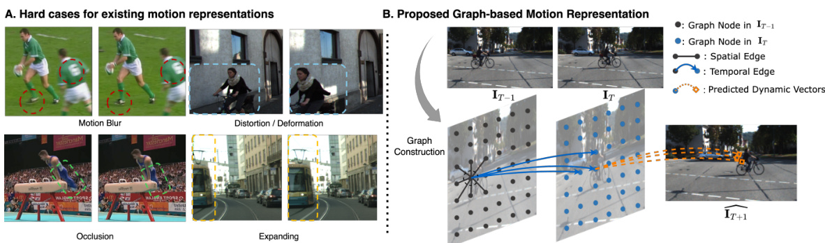
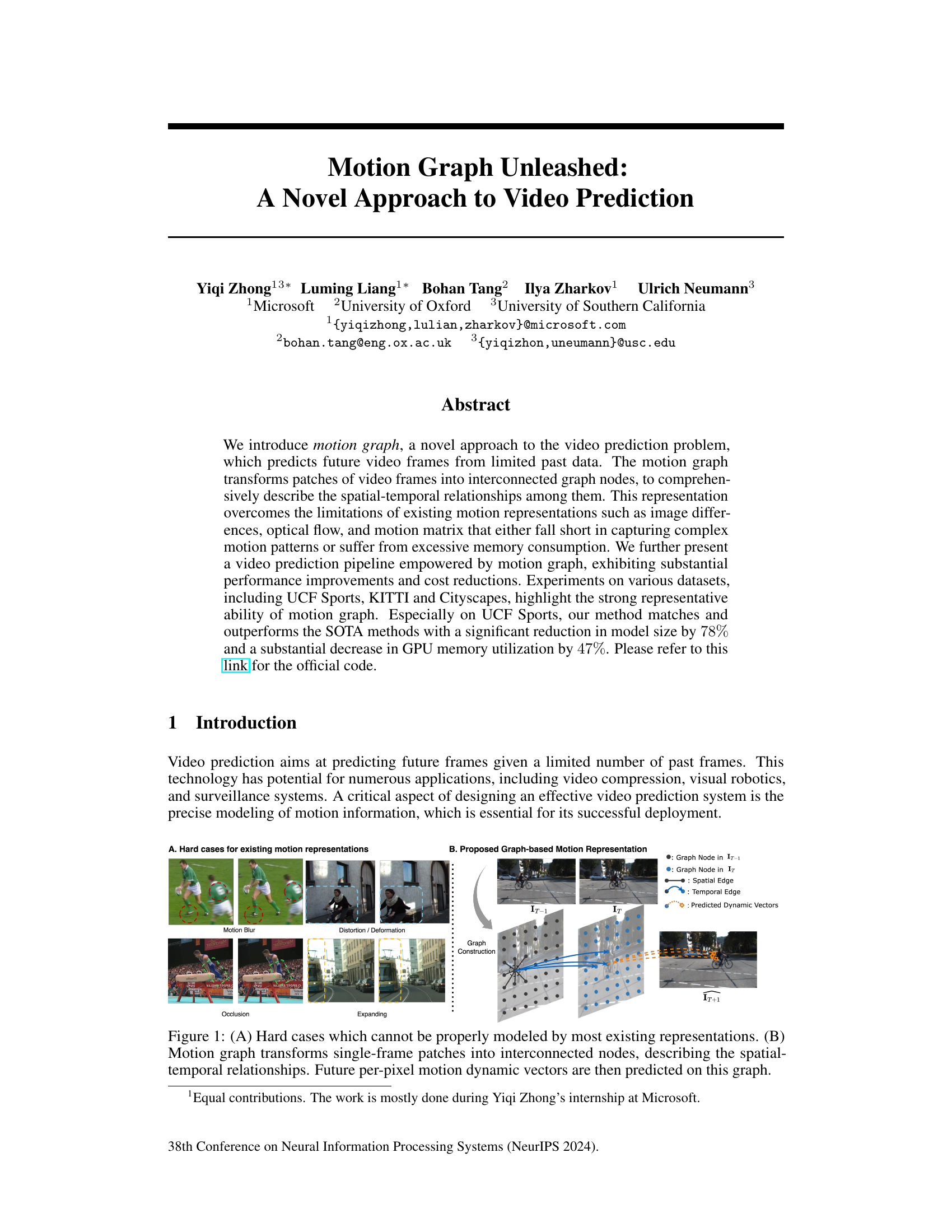
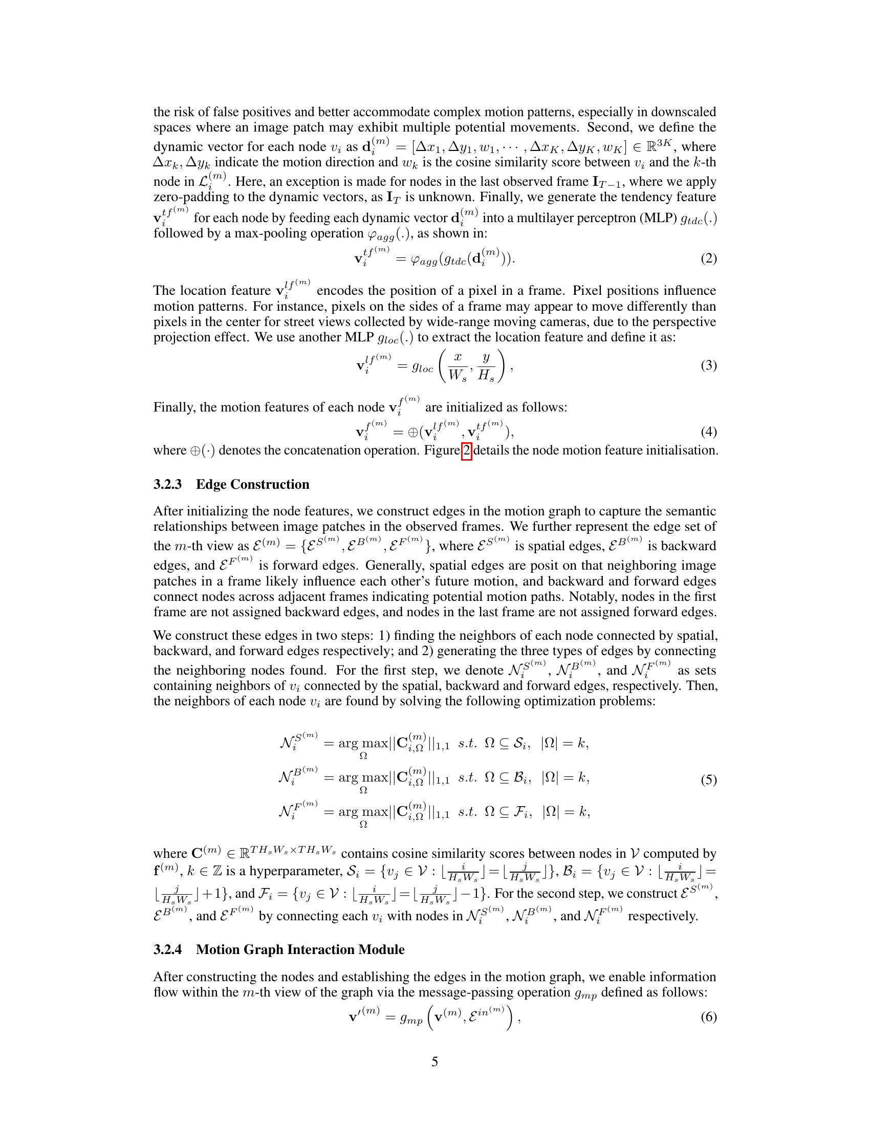
This figure demonstrates the challenges of existing motion representations and introduces the proposed motion graph. Part (A) showcases scenarios that are difficult for existing methods to model accurately, including motion blur, distortion/deformation, occlusion, and expansion. Part (B) illustrates the motion graph, a novel approach where video frames are broken into patches (nodes) interconnected based on their spatial-temporal relationships. The future motion of each pixel is predicted using this graph.
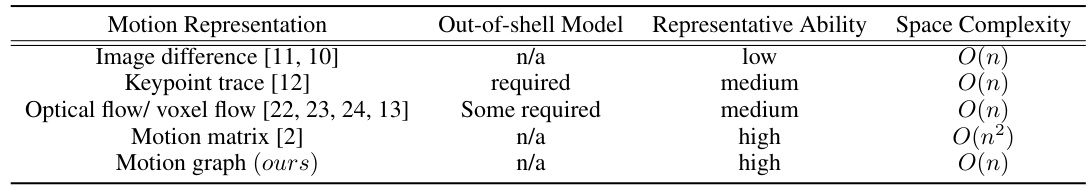
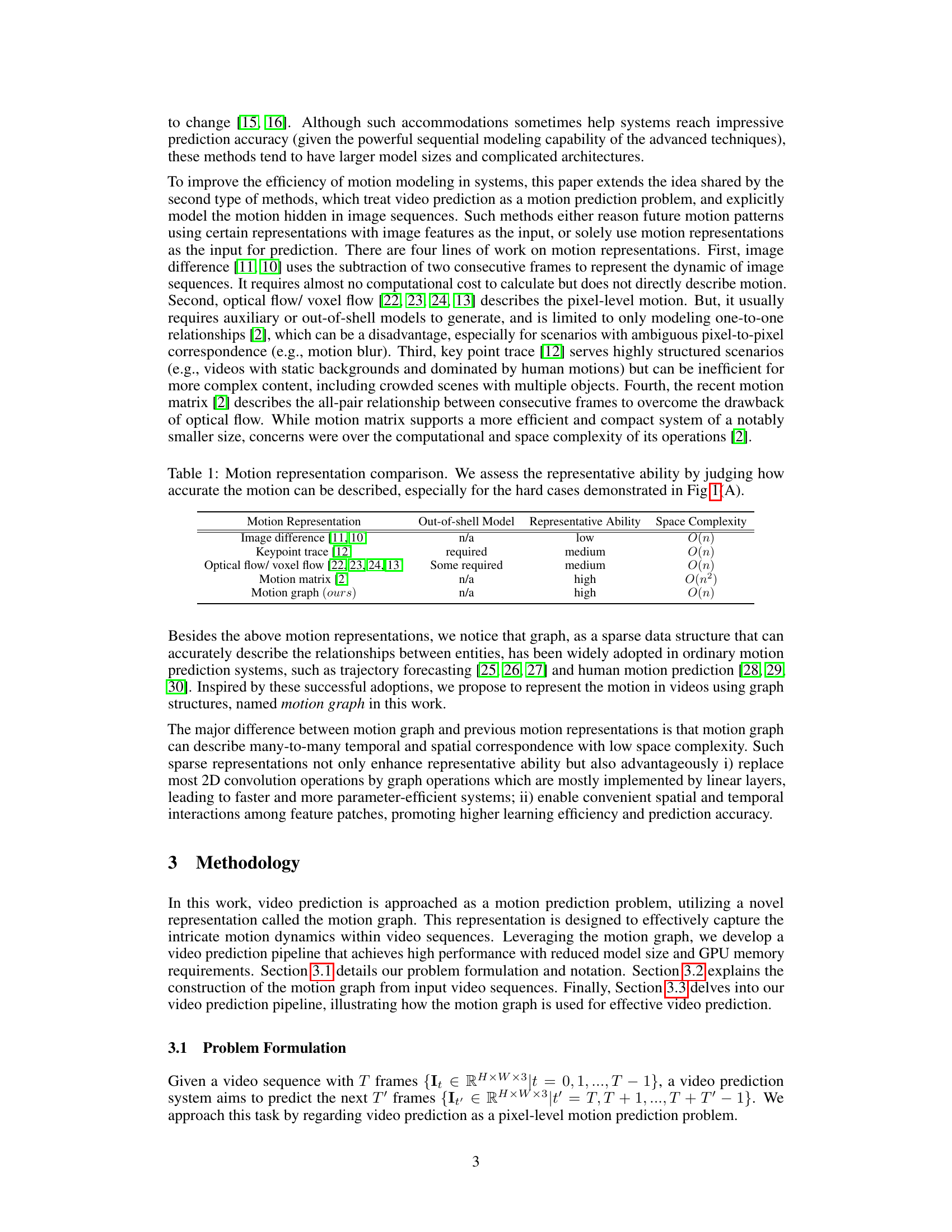
This table compares different motion representations used in video prediction, namely image difference, keypoint trace, optical flow/voxel flow, motion matrix, and the proposed motion graph. For each method, it indicates whether an external model is needed to generate the motion representation, its ability to represent complex motion patterns (representative ability), and its space complexity. The table highlights that while the motion matrix has high representative ability, it also has a high space complexity; conversely, the proposed motion graph offers a good balance between representative ability and space efficiency.
In-depth insights#
Motion Graph Model#
The Motion Graph Model, as described in the research paper, presents a novel approach to video prediction by leveraging the power of graph neural networks. It ingeniously transforms video frames into interconnected graph nodes representing patches of frames, where each node encapsulates spatial-temporal relationships. This graph structure offers significant advantages over traditional methods like optical flow and motion matrices, effectively capturing complex motion patterns while maintaining computational efficiency. The use of dynamic vectors associated with each node further enhances the model’s representational power. These vectors predict future per-pixel motion, offering a granular approach to video frame prediction. By cleverly interweaving spatial and temporal edges in the graph, the model successfully integrates spatial-temporal context for motion prediction. The graph structure allows for parallel processing of information, significantly improving computation speed. Experimental results indicate that the Motion Graph Model achieves state-of-the-art performance on multiple datasets, while requiring substantially less GPU memory and model size, showcasing its effectiveness and efficiency. The model’s success underscores the potential of graph neural networks for complex sequence prediction tasks like video prediction. However, its performance may vary on videos with abrupt motion or occlusions, posing avenues for future research and optimization.
Video Prediction Pipeline#
A video prediction pipeline, at its core, aims to forecast future video frames based on a limited set of past frames. This process typically involves several key stages: motion estimation, which accurately captures how objects and scenes move in the video; motion representation, converting the motion data into a suitable format for prediction (e.g., optical flow, motion graphs); a prediction model, which learns patterns from the motion data and predicts future frames; and frame generation, which transforms the prediction into a visual format. The success of a video prediction pipeline hinges heavily on the accuracy of the motion estimation and representation, as well as the predictive power of the chosen model. Moreover, efficiency and scalability are critical considerations, particularly with higher-resolution videos, requiring optimal memory and computational resource management. Advanced techniques like deep learning models are often incorporated, but simpler, more efficient methods are always under investigation for real-world applications demanding speed and minimal resource usage. The ultimate goal is to generate realistic and accurate video predictions that are indistinguishable from real footage.
Experimental Results#
The experimental results section of a research paper is crucial for validating the claims and demonstrating the effectiveness of proposed methods. A strong results section should present findings clearly and comprehensively, using appropriate visualizations such as graphs and tables. Quantitative metrics, such as precision, recall, F1-score, or accuracy, should be reported with error bars to show statistical significance. Qualitative analysis may be included to provide deeper insights, but it should be objective and supported by data. The results should be presented in a way that is easy for the reader to interpret and should be compared to existing state-of-the-art methods. It’s vital to discuss the implications of the results, including potential limitations and areas for future work. Careful consideration of experimental design is crucial to ensure the validity and reliability of the reported results. This includes aspects like data splitting, handling bias, and proper controls. A thorough presentation of experimental results increases the credibility and impact of the research paper.
Computational Efficiency#
The research paper highlights significant advancements in computational efficiency for video prediction. This is achieved primarily through the introduction of a novel motion representation called “motion graph.” Unlike traditional methods that use computationally expensive techniques like dense optical flow or high-dimensional motion matrices, the motion graph transforms video frames into a sparse graph structure. This sparse representation dramatically reduces the computational burden, resulting in substantial cost reductions. Experiments reveal that the motion graph-based approach not only matches the state-of-the-art in prediction accuracy but also achieves a remarkable 78% reduction in model size and 47% decrease in GPU memory utilization. The efficiency gains stem from the graph’s inherent sparsity, enabling more efficient message-passing operations compared to traditional convolutional approaches. This highlights the potential of graph-based models for resource-constrained environments and makes the proposed method particularly appealing for real-time applications. The key contributions are therefore both accuracy improvement and significantly decreased resource demands, making this approach practical for real world applications.
Future Research#
Future research directions stemming from this motion graph-based video prediction model could explore several avenues. Improving inference speed is crucial, potentially through architectural optimizations or specialized hardware acceleration. Addressing limitations in handling sudden or unpredictable movements warrants further investigation, perhaps by incorporating more robust motion representation techniques or employing attention mechanisms that focus on relevant details. Expanding to long-term video prediction presents a significant challenge but offers substantial rewards, necessitating the development of more sophisticated temporal modeling. Investigating the potential for generalization across diverse video domains and evaluating performance with variations in resolution, lighting, and camera motion is essential. Finally, exploring the applications of the motion graph in other areas beyond video prediction, such as object tracking, action recognition, and visual robotics is promising. Addressing limitations in handling occlusions and complex scenes also requires attention. The efficacy of the motion graph architecture should be tested on challenging real-world data, enhancing its robustness and practicality.
More visual insights#
More on figures
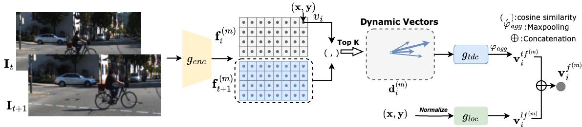
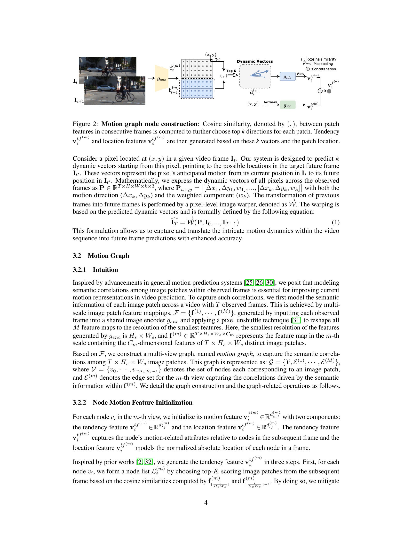
This figure illustrates the process of constructing a node in the motion graph. It starts with computing cosine similarity between patch features from consecutive frames (It and It+1) to identify the top k most likely motion directions for each patch. These directions, along with the patch’s location, are used to generate the tendency (tf(m)) and location (lf(m)) features for the node, which represent the node’s motion-related attributes and its spatial position within the frame, respectively. These features are then combined to form the final node motion feature (vf(m)).
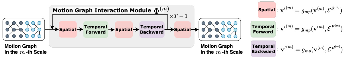
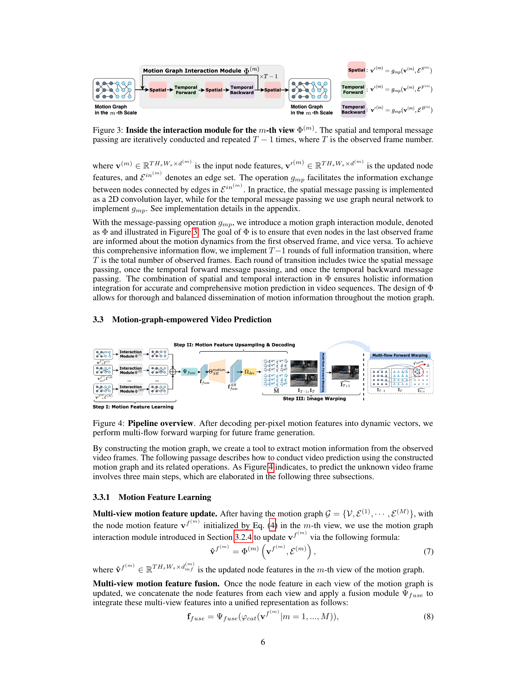
This figure illustrates the inner workings of the motion graph interaction module. The spatial message passing is shown as a 2D convolution, while temporal message passing utilizes a graph neural network. The process iterates T-1 times (where T is the number of observed frames), alternating between spatial and temporal message passing (forward and backward). The goal is to ensure complete information flow across all frames, even influencing the last frame’s nodes with information from the beginning.
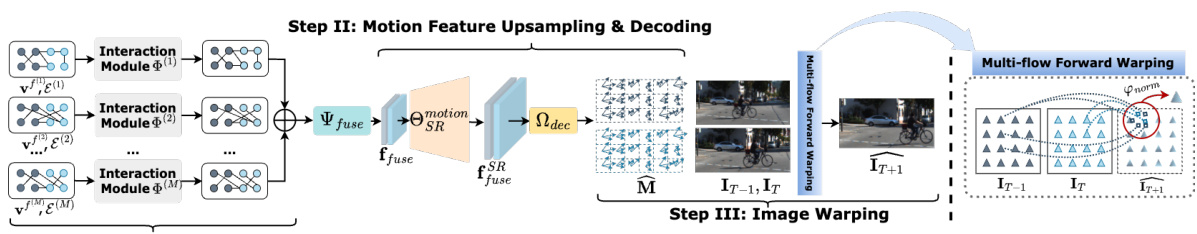
This figure illustrates the three main steps of the video prediction pipeline using motion graphs. Step I shows the process of learning motion features from the observed video frames using multiple motion graph interaction modules. The motion features from different scales are fused to create a unified representation. Step II involves upsampling the motion features to the original image resolution using a motion upsampler (OSR) and decoding them into dynamic vectors using a motion decoder (Ωdec). Finally, step III performs the multi-flow forward warping to generate the predicted future frame from the past frames and the dynamic vectors, resulting in the synthesis of future frames (IT+1).
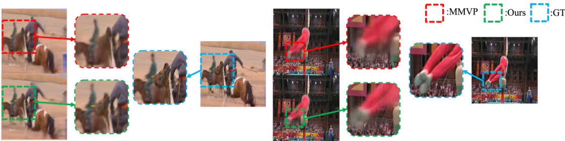
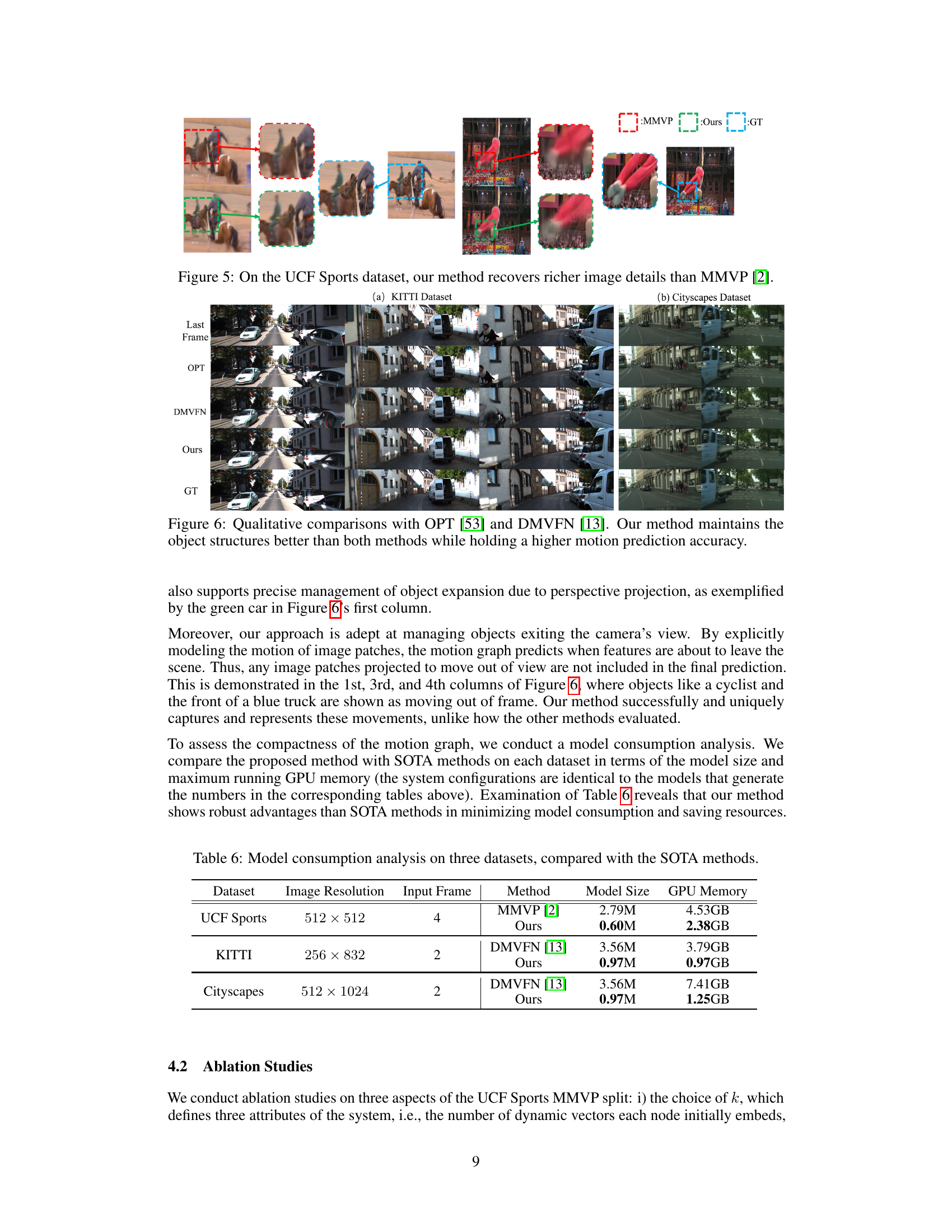
This figure presents a qualitative comparison of video prediction results between the proposed method and MMVP on the UCF Sports dataset. It showcases that the proposed method, compared to MMVP, better preserves the details of the image. This improved detail preservation is particularly noticeable in areas with complex motion or blurring, suggesting that the proposed method is superior in handling challenging motion scenarios.
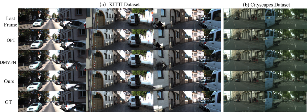
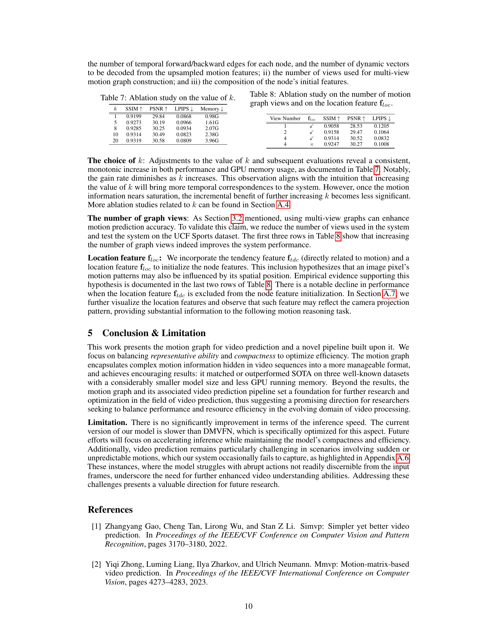
This figure shows a qualitative comparison of video prediction results between the proposed method and two state-of-the-art methods (OPT and DMVFN) on KITTI and Cityscapes datasets. The results demonstrate that the proposed method better preserves object structures and achieves higher motion prediction accuracy compared to the other methods, especially in handling perspective effects and occlusions. Each column represents a different video sequence, showing the last observed frame, predictions by OPT, DMVFN, the proposed method, and the ground truth (GT).
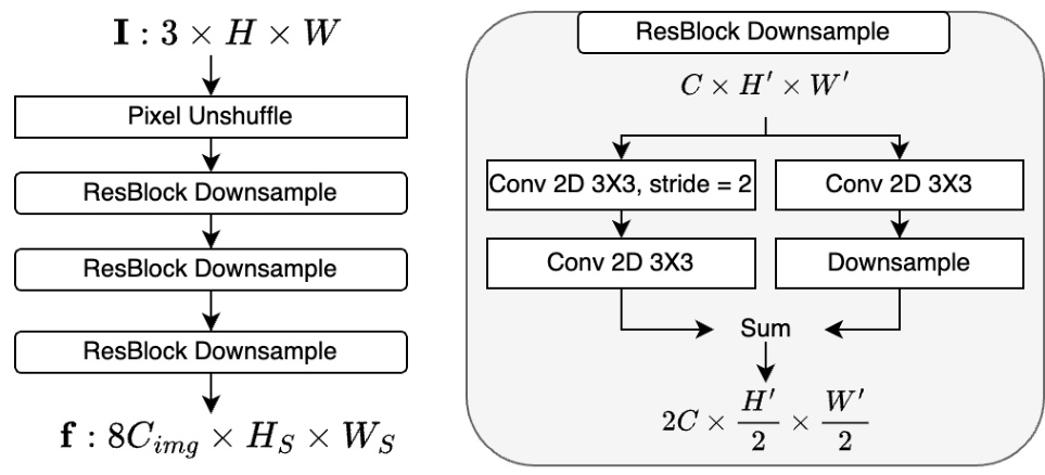
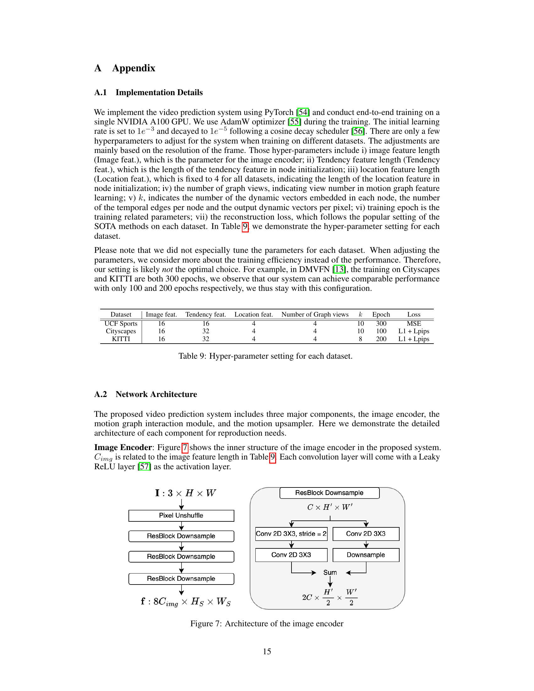
The image encoder consists of four ResBlock Downsample layers followed by a pixel unshuffle layer. The ResBlock Downsample layers use a combination of convolutional layers, downsampling, and residual connections to extract multi-scale features from the input image (3 x H x W). The pixel unshuffle layer reshapes the output feature maps to the desired resolution (8Cimg x Hs x Ws).
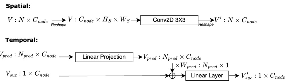
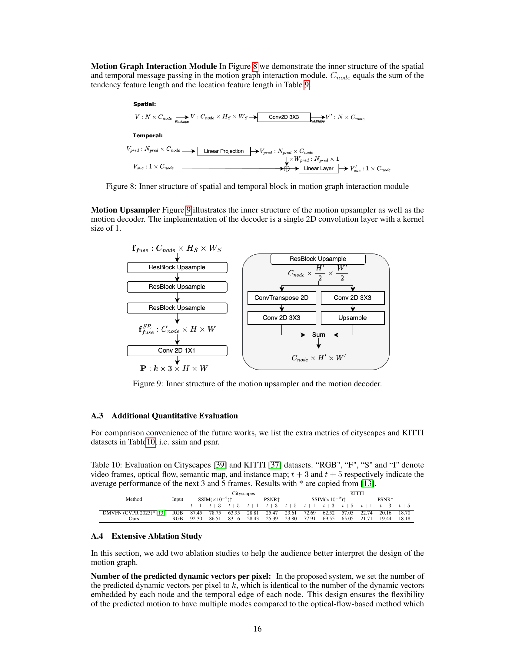
This figure shows the architecture of the spatial and temporal message passing within the motion graph interaction module. The spatial message passing uses a 2D convolution to update node features based on spatial relationships. The temporal message passing involves a linear projection to create prediction vectors from previous nodes, and a linear layer to combine these predictions with information from the successor nodes.
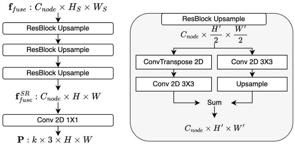
This figure shows the architecture of the motion upsampler and decoder used in the video prediction pipeline. The upsampler takes the fused multi-view motion features (ffuse) as input and progressively increases the resolution using ResBlock Upsample layers to match the original video frame resolution (H x W). Finally, a 1x1 convolution layer converts the upsampled features into dynamic vectors (P) representing pixel-level motion.
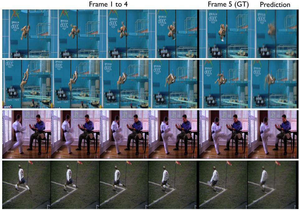
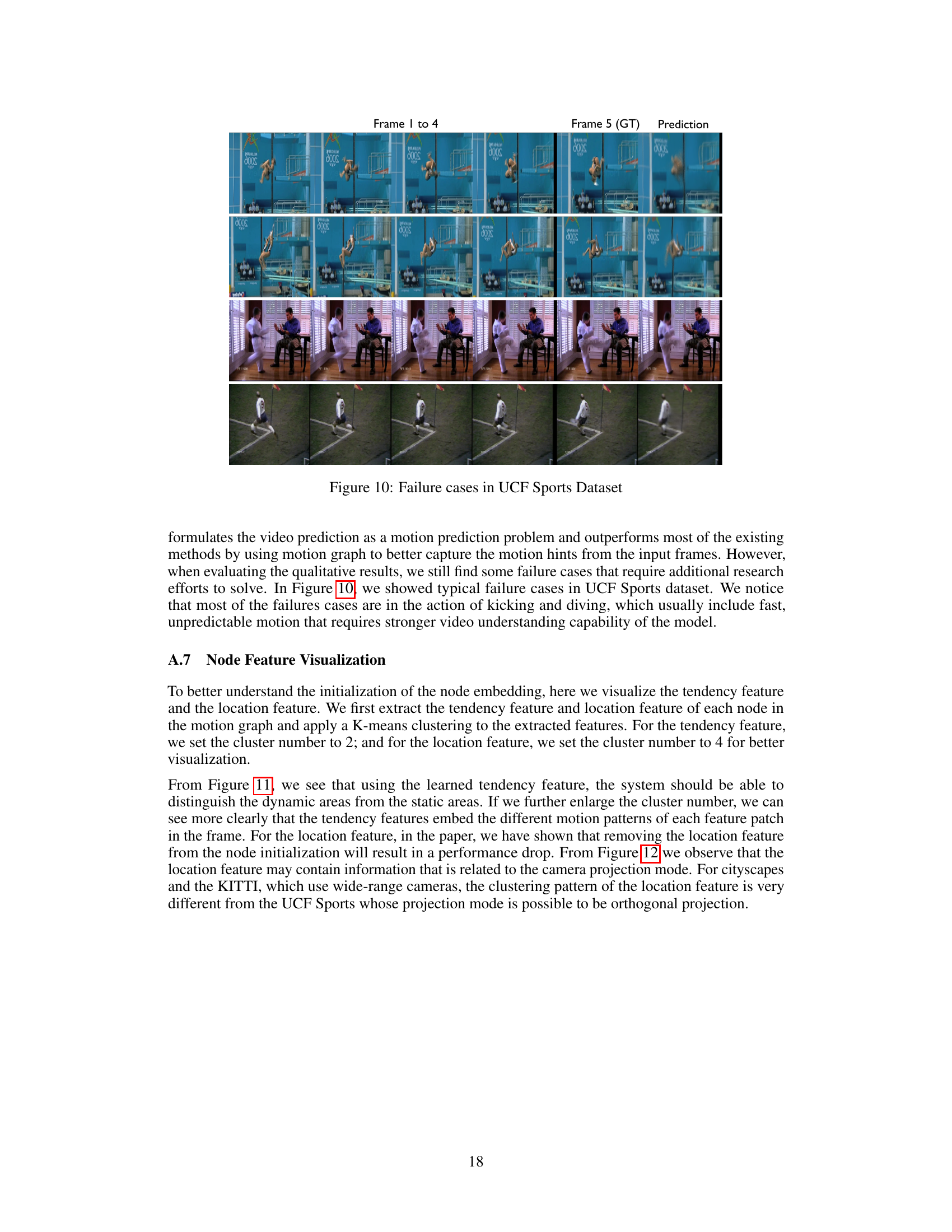
This figure showcases examples where the video prediction model struggles. The examples depict scenarios involving fast, unpredictable movements such as kicking and diving. These actions present challenges for the model’s ability to accurately predict future frames due to their dynamic and less easily predictable nature. The figure visually demonstrates limitations of the approach when confronted with complex and sudden motion, highlighting areas for future improvements.
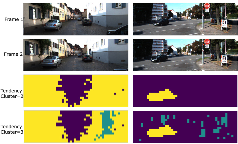
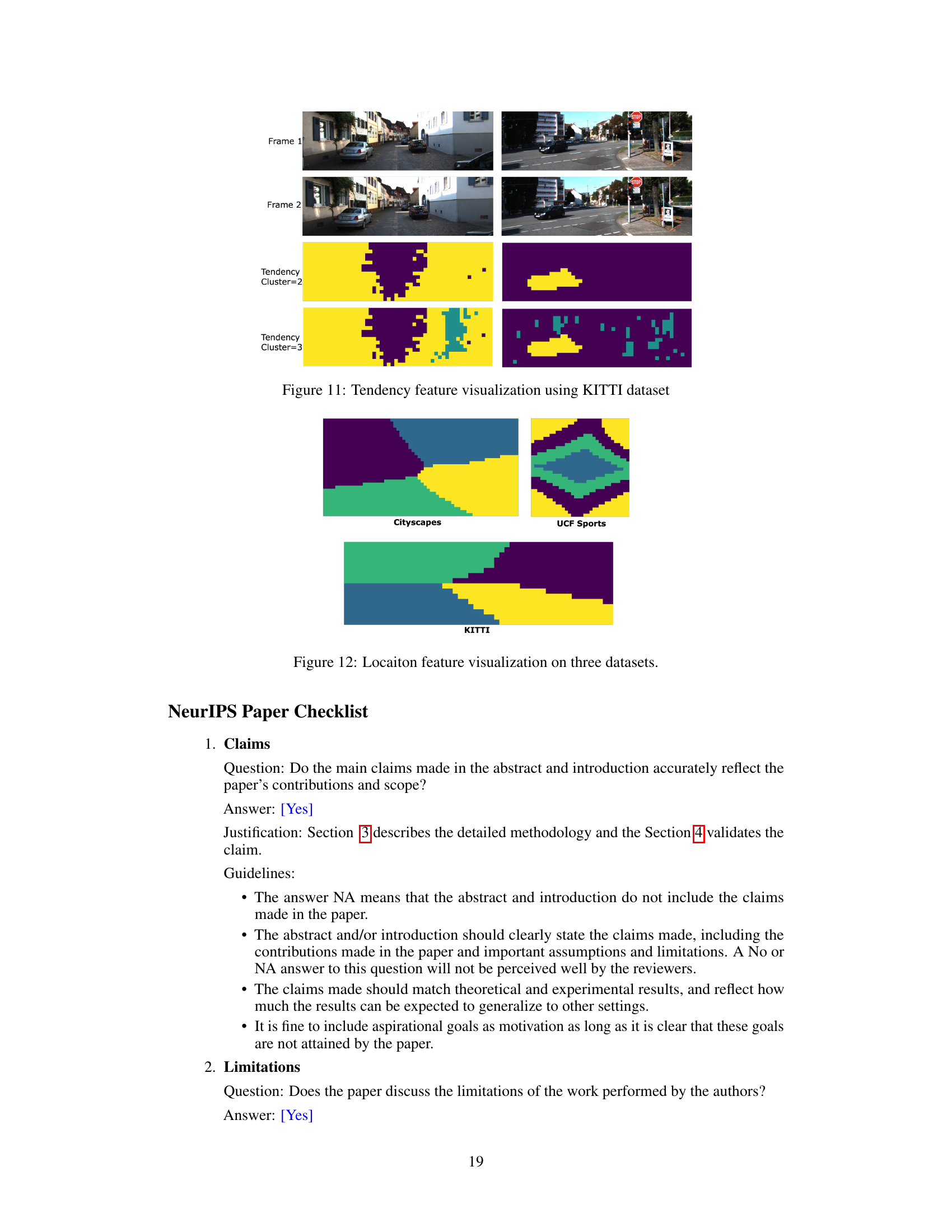
This figure visualizes the tendency features extracted from the KITTI dataset using K-means clustering. The top row shows example frames from the dataset. The bottom two rows display the results of the clustering, using 2 and 3 clusters respectively. Each color represents a cluster, indicating different motion patterns detected by the model within the image patches. Areas of similar motion are grouped into the same color. The visualization demonstrates the model’s ability to differentiate between static and dynamic regions of the frames, and its capability of clustering similar movement patterns together.
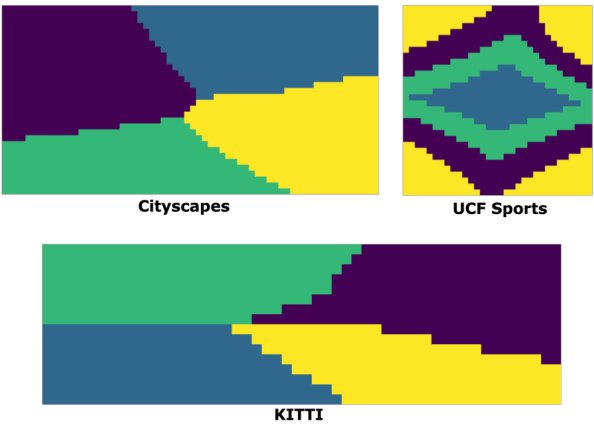
This figure visualizes the location features extracted from three different datasets: Cityscapes, UCF Sports, and KITTI. The location feature represents the spatial position of image patches. A K-means clustering algorithm was applied to the location features, resulting in a color-coded visualization showing the distribution of the spatial patterns. The differences in the patterns across datasets demonstrate the varying characteristics of these datasets.
More on tables
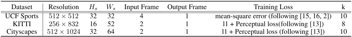
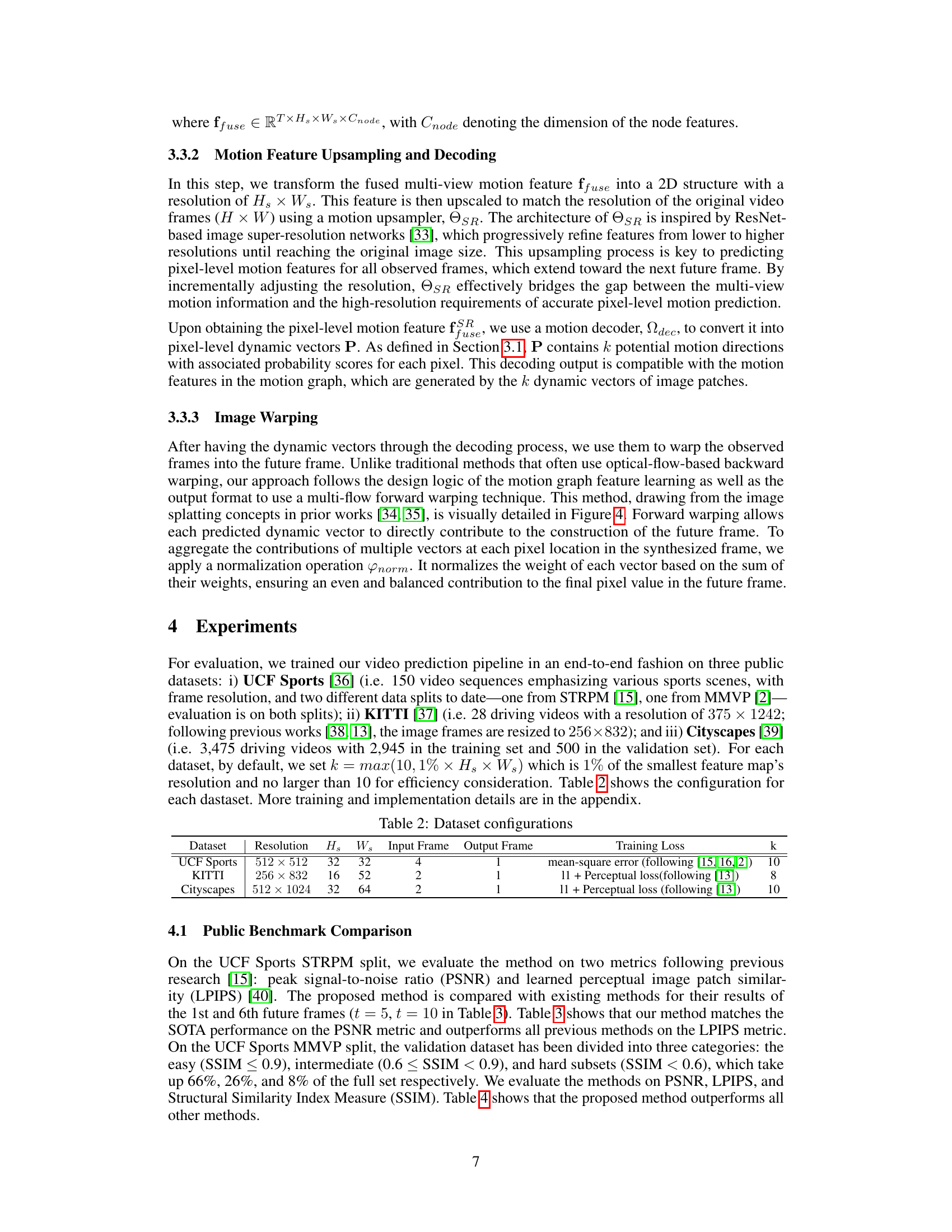
This table presents the configurations used for each dataset in the video prediction experiments. It shows the resolution of the images, the size of the smallest feature maps (Hs and Ws), the number of input frames used for prediction, the number of output frames predicted, the type of loss function used during training, and the hyperparameter k (which influences the number of dynamic vectors, temporal edges per node, and output dynamic vectors per pixel).
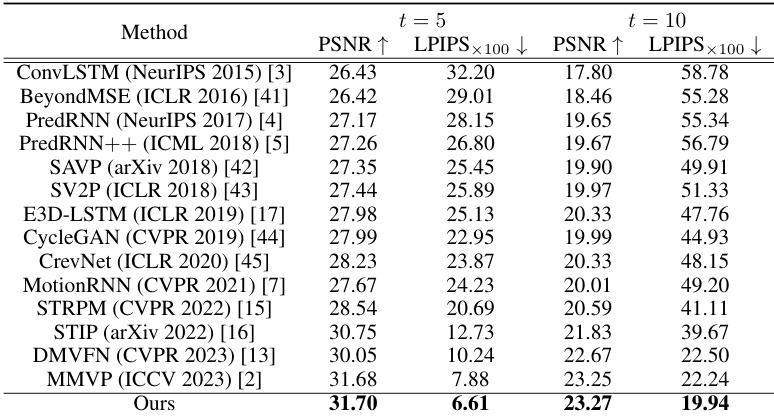
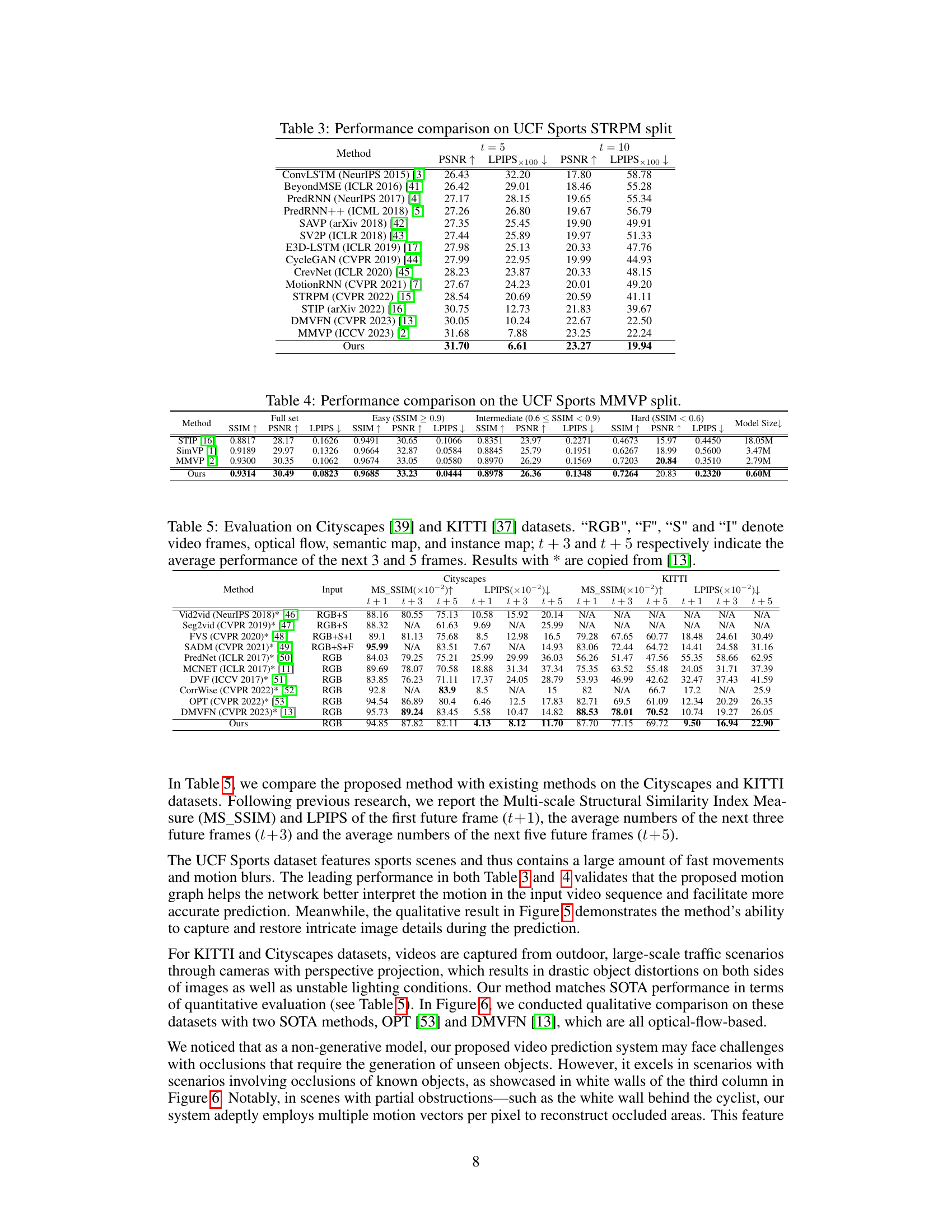
This table compares the performance of the proposed method with other state-of-the-art (SOTA) methods on the UCF Sports STRPM split dataset. The performance is evaluated using two metrics: Peak Signal-to-Noise Ratio (PSNR) and Learned Perceptual Image Patch Similarity (LPIPS). Results are shown for both the 5th (t=5) and 10th (t=10) future frames, providing a comprehensive comparison across various methods.
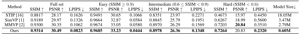
This table presents a performance comparison of different video prediction methods on the UCF Sports MMVP dataset split into three categories based on the structural similarity index (SSIM) score: easy (SSIM ≥ 0.9), intermediate (0.6 < SSIM < 0.9), and hard (SSIM < 0.6). The metrics used for comparison include SSIM, PSNR, and LPIPS for each category and the full dataset. The model sizes of each method are also listed, demonstrating the efficiency of the proposed approach.
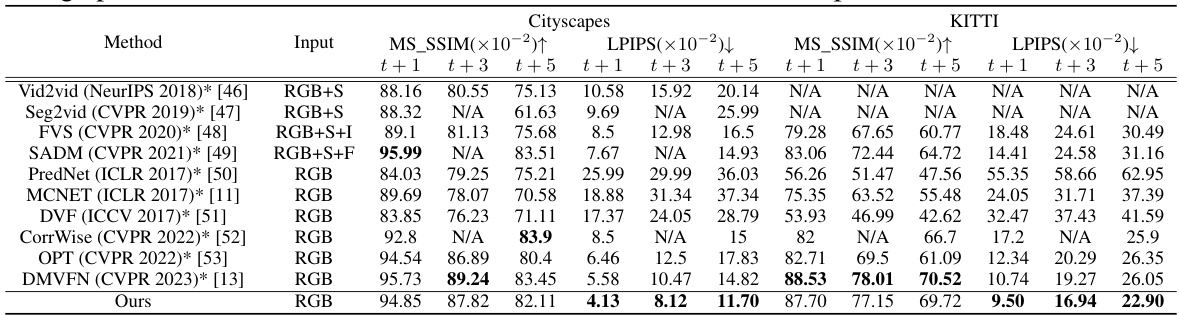
This table presents a quantitative comparison of the proposed method with other state-of-the-art video prediction methods on the Cityscapes and KITTI datasets. The evaluation metrics include Multi-scale Structural Similarity Index Measure (MS-SSIM) and Learned Perceptual Image Patch Similarity (LPIPS) for different prediction horizons (t+1, t+3, t+5 frames). The input modalities used in each method are also listed (RGB, optical flow (F), semantic map (S), instance map (I)).
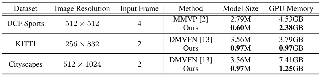
This table compares the model size and GPU memory usage of the proposed method with state-of-the-art (SOTA) methods on three datasets: UCF Sports, KITTI, and Cityscapes. It highlights the significant reduction in model size and GPU memory utilization achieved by the proposed approach, demonstrating its efficiency.
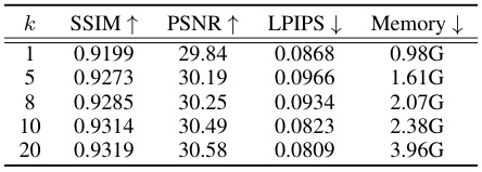
This table presents the ablation study on the impact of the hyperparameter k on the performance of the video prediction model. The hyperparameter k controls multiple aspects of the model: the number of dynamic vectors each node initially embeds, the number of temporal forward/backward edges for each node, and the number of dynamic vectors to be decoded from the upsampled motion features. The table shows the SSIM, PSNR, LPIPS, and GPU memory usage for different values of k (1, 5, 8, 10, and 20). It demonstrates how changing k affects the balance between performance and resource consumption.
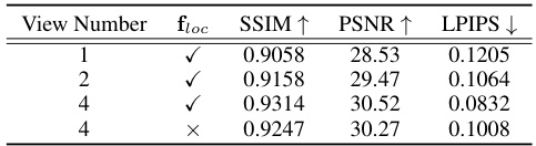
This table presents the results of ablation studies conducted to evaluate the impact of the number of motion graph views and the inclusion of the location feature (floc) on the model’s performance. The study assesses the effect on SSIM, PSNR, and LPIPS metrics. The results show that increasing the number of views improves performance, while excluding the location feature leads to a decrease in performance.
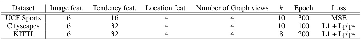
This table shows the configuration settings used for each dataset in the video prediction experiments. It lists the resolution of the input videos, the size of the smallest feature maps (Hs x Ws) generated by the image encoder, the number of input frames used for prediction, the number of output (predicted) frames, the type of loss function used during training, and the value of the hyperparameter ‘k’. The ‘k’ value determines several aspects of the model, including the number of dynamic vectors per node in the motion graph, the number of temporal edges per node, and the number of dynamic vectors per pixel in the output.
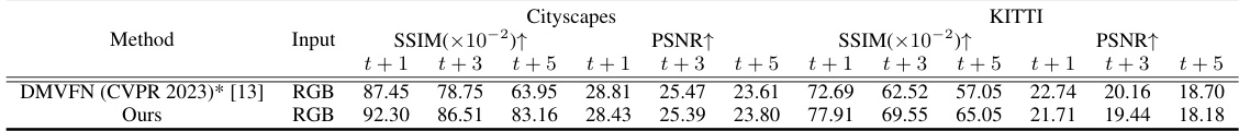
This table presents a comparison of the proposed method’s performance against existing methods on the Cityscapes and KITTI datasets for video prediction. It shows the Multi-scale Structural Similarity Index Measure (MS-SSIM) and Peak Signal-to-Noise Ratio (PSNR) for the first frame (t+1), the average of the next three frames (t+3), and the average of the next five frames (t+5). The input modalities used are also specified (RGB, RGB+F, RGB+S, RGB+S+I, RGB+S+F). Results marked with * are taken directly from the cited DMVFN paper.
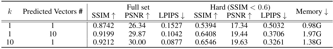
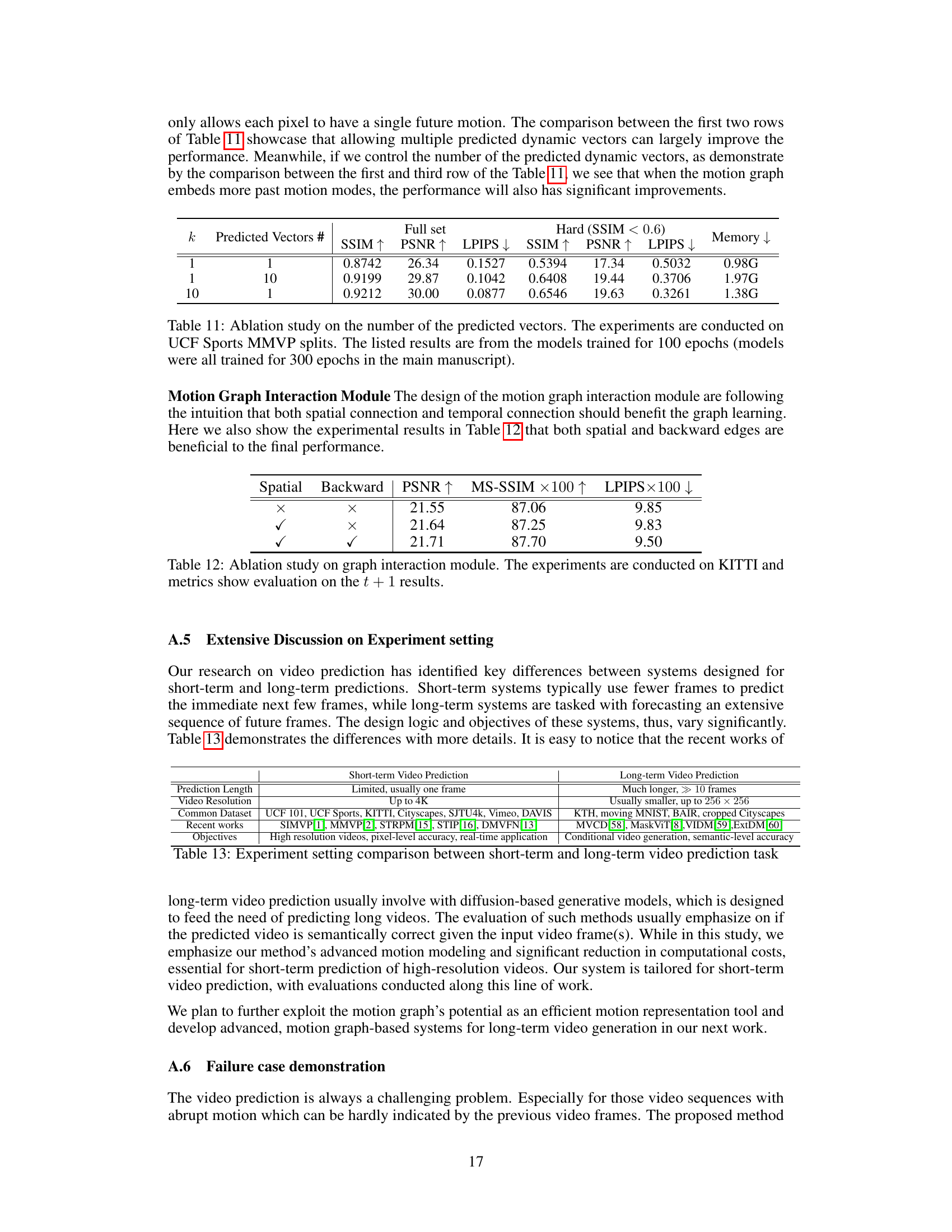
This table presents the ablation study result on the number of predicted vectors used in the model. It shows the impact of varying the number of predicted vectors (k) on the model’s performance, measured by SSIM, PSNR, and LPIPS metrics. The study was conducted on the UCF Sports MMVP dataset split, and results are shown for both the full dataset and the subset with SSIM less than 0.6. Memory consumption is also listed to indicate the efficiency of the model with different k values.
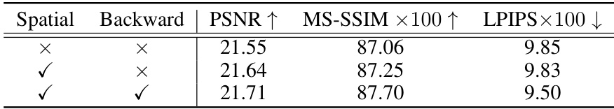
This table presents the ablation study results on the KITTI dataset for the motion graph interaction module. It shows the impact of using spatial edges, backward edges, and both on the performance metrics PSNR, MS-SSIM, and LPIPS for predicting the next frame (t+1). The results demonstrate that incorporating both spatial and temporal information significantly improves the video prediction accuracy.
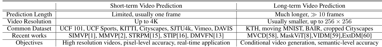
This table compares different motion representation methods used in video prediction, including image difference, keypoint trace, optical flow/voxel flow, motion matrix, and the proposed motion graph. For each method, it indicates whether an out-of-shell model is required, its representative ability (assessed by how well it captures complex motions), and its space complexity. The table highlights the advantages of the motion graph in terms of representational power and efficiency.
Full paper#