↗ OpenReview ↗ NeurIPS Homepage ↗ Hugging Face ↗ Chat
TL;DR#
Large Language Models (LLMs) struggle to generate highly structured outputs like code or formulas while adhering to grammatical constraints. Current methods, like grammar-constrained decoding (GCD), often distort the LLM’s probability distribution, leading to grammatically correct but low-quality outputs. This is because GCD greedily restricts the LLM’s output to only grammatically valid options without considering the true probability of those options according to the LLM.
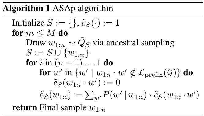
This paper introduces a new method called Grammar-Aligned Decoding (GAD) to address these limitations. The proposed algorithm, Adaptive Sampling with Approximate Expected Futures (ASAp), uses past samples to iteratively improve approximations of the LLM’s probability distribution conditioned on the grammar constraints. It starts as a GCD method but gradually converges to the true distribution. Evaluation on various tasks shows ASAp generates outputs with higher likelihood and better respects the LLM’s distribution than existing methods, demonstrating significant improvements in the quality of structured outputs.
Key Takeaways#
Why does it matter?#
This paper is crucial because it addresses a critical limitation in current large language model (LLM) applications: the distortion of LLM distributions by existing constrained decoding methods. By introducing a novel algorithm, ASAp, the research directly tackles this problem and improves the quality of structured outputs significantly. This opens new avenues for enhancing various LLM applications requiring structured generation. The rigorous theoretical analysis and compelling empirical results will shape future work in constrained decoding.
Visual Insights#

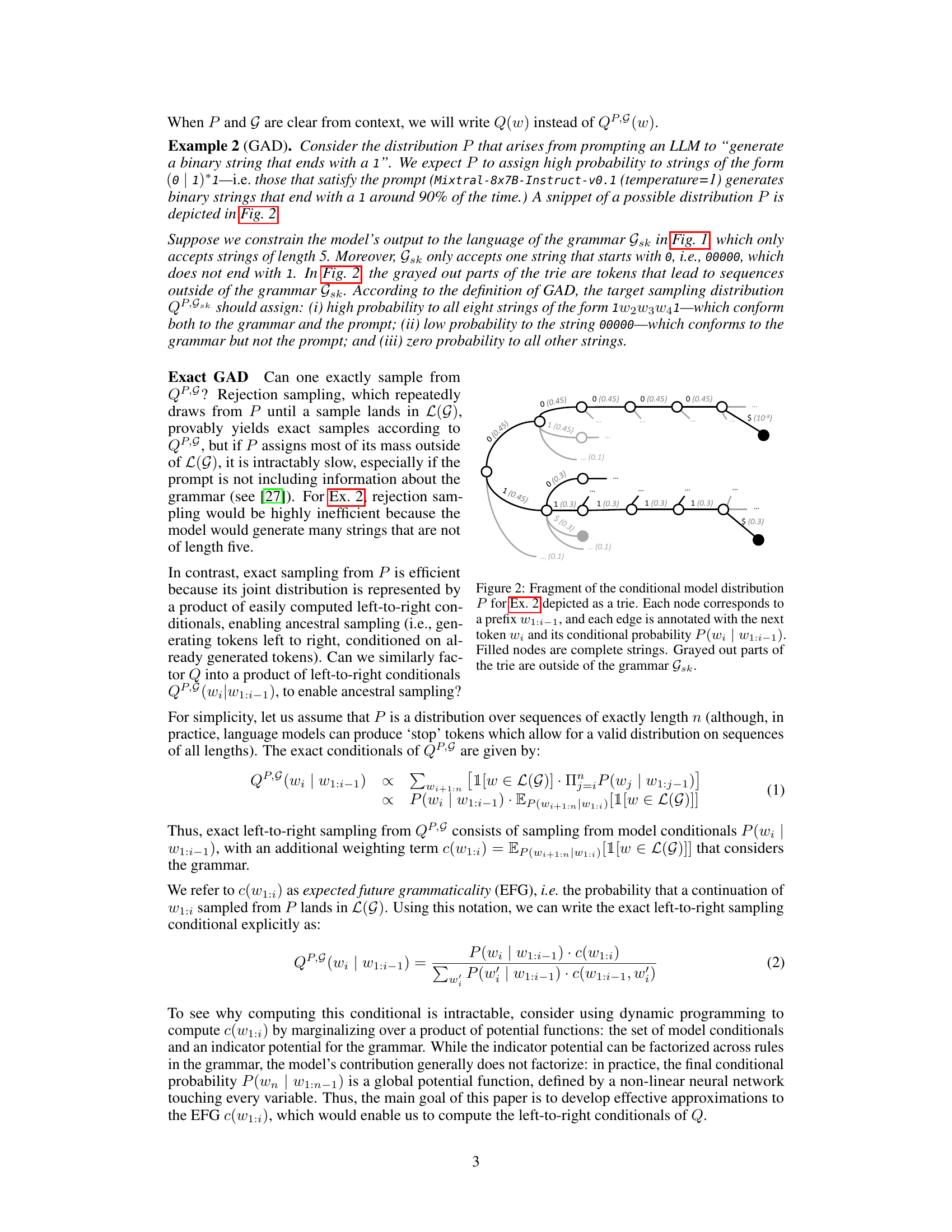
This figure shows a fragment of a conditional model distribution, represented as a trie data structure. Each node in the trie represents a prefix of a string, and each edge represents a token with its conditional probability given the prefix. Filled nodes represent complete strings which are accepted by the model. Grayed-out portions of the trie show prefixes that are not part of the grammar Gsk, highlighting how the model’s distribution is different than the desired grammar-constrained distribution. This illustrates the challenge in aligning sampling with a grammar constraint, which is the central problem addressed in the paper.
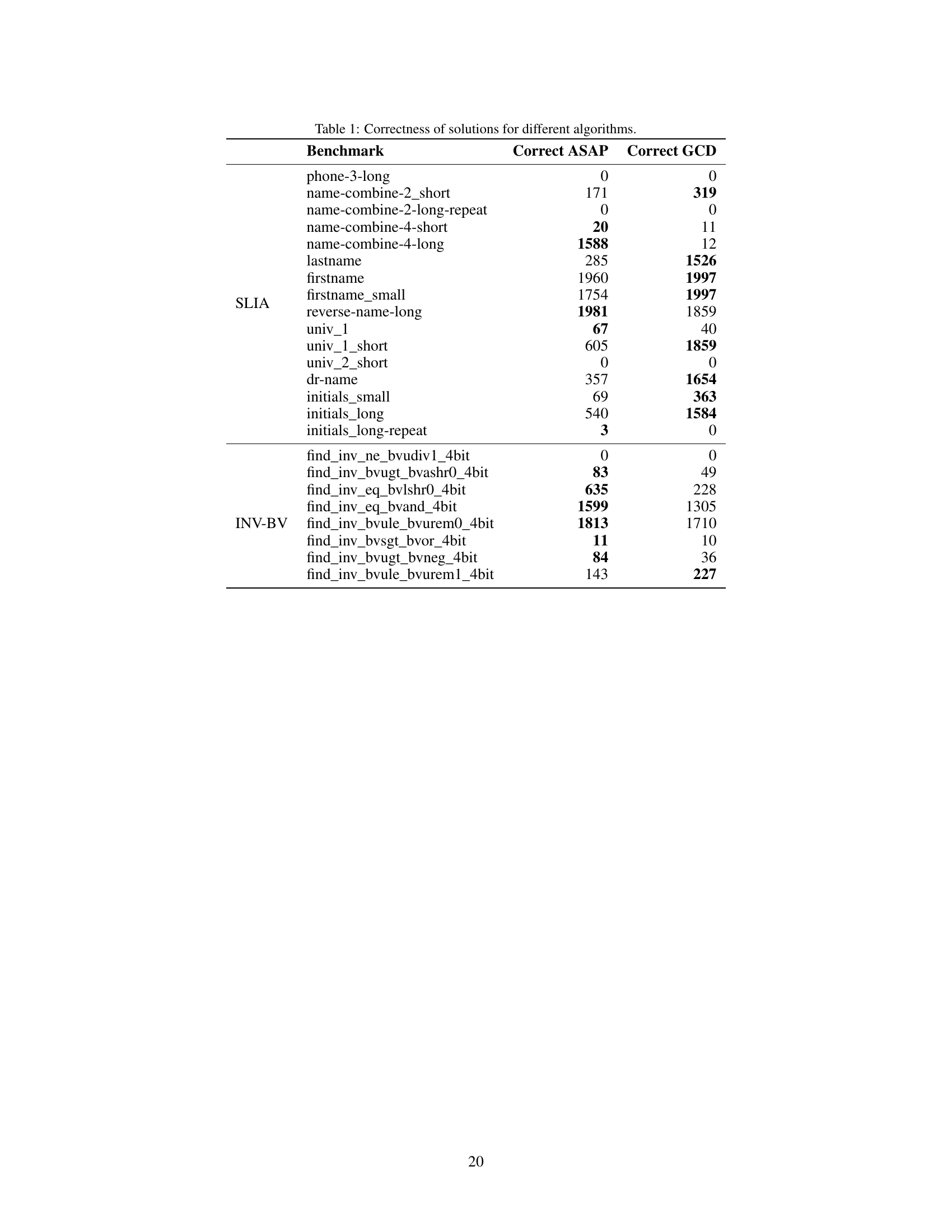
This table presents the number of correct solutions obtained by ASAp and GCD for various benchmarks across different structured prediction tasks. It compares the performance of the two algorithms in terms of generating grammatically correct outputs that satisfy given constraints. The benchmarks include different variations of string manipulation tasks (SLIA) and bit-vector arithmetic problems (INV-BV). Higher numbers indicate better performance.
In-depth insights#
LLM Struct Gen#
LLM Struct Gen, a hypothetical heading, likely refers to the generation of structured text using Large Language Models (LLMs). This area is crucial because while LLMs excel at generating fluent text, they often struggle with maintaining consistent structure, a critical aspect for applications demanding precise formatting like code, formulas, or markup. The core challenge lies in aligning the probabilistic nature of LLM outputs with the rigid rules defining structure. This could involve techniques like grammar-constrained decoding, which ensures grammaticality but might distort the LLM’s natural distribution, leading to lower-quality results, or novel methods seeking to seamlessly merge probabilistic generation with structural constraints. Research in this area is likely exploring novel decoding algorithms, improved grammar formalisms, and perhaps even architectural changes to LLMs themselves to better facilitate structured generation. The ultimate goal is to leverage the power of LLMs for generating diverse and creative structured content while maintaining the fidelity and quality expected from structured data.
GAD Formalism#
A hypothetical section titled ‘GAD Formalism’ in a research paper would rigorously define grammar-aligned decoding (GAD). It would likely begin by formally stating the problem: sampling from a language model’s distribution while strictly adhering to a given grammar. The formalism would then introduce notation for relevant concepts—the language model’s probability distribution P, the context-free grammar G, and its language L(G). Crucially, it would define the target distribution Q, which represents the desired GAD outcome: a probability distribution proportional to P but restricted to strings within L(G). The section would mathematically characterize the relationship between P and Q, perhaps demonstrating the intractability of exact sampling from Q. This would set the stage for the subsequent introduction of approximate algorithms, justifying their necessity and providing a formal benchmark for their evaluation. Key elements of the formalism might include the definition of expected future grammaticality (EFG), representing the probability of completing a given prefix into a valid grammatical sentence according to P. The complexity of calculating EFG directly might be discussed, highlighting the need for approximation techniques. Finally, the section could explicitly address how its defined formalism relates to and improves upon existing methods like grammar-constrained decoding (GCD), clearly articulating the novel contributions and improvements of the proposed GAD approach.
ASAP Algorithm#
The core of the research paper revolves around the Adaptive Sampling with Approximate Expected Futures (ASAP) algorithm, designed to address the limitations of existing grammar-constrained decoding (GCD) methods in language model sampling. ASAP’s key innovation is its iterative approach, which starts with a GCD-like strategy but progressively refines its sampling distribution by incorporating information from previously generated samples. This iterative refinement, based on the concept of approximate expected futures, helps to reduce bias in sampling, ensuring outputs closely align with the original language model’s distribution while still adhering to grammatical constraints. The algorithm leverages learned approximations of the probability of future grammaticality, dynamically updating these probabilities as more samples become available. This adaptive mechanism is crucial for mitigating the distortion effects often observed in GCD, where grammaticality constraints can significantly skew the sampling process, leading to outputs that are grammatically correct but improbable under the original model. The theoretical analysis of the algorithm’s convergence behavior and empirical evaluations on code generation and natural language processing tasks demonstrates ASAP’s superior ability to produce high-likelihood, grammatically-correct outputs compared to GCD, highlighting its significance in addressing the challenges of generating highly structured outputs from large language models.
Empirical Results#
An Empirical Results section would ideally present a detailed analysis of experimental findings, comparing the proposed ASAp algorithm against existing GCD techniques. Key aspects to cover include quantitative metrics such as KL divergence to measure the alignment between the sampled distribution and the true LLM distribution, conditioned on the grammar. The results should show that ASAp converges towards the target distribution, better respecting the LLM’s probabilities while maintaining grammatical constraints. Visualizations like plots of KL divergence over iterations or expectation comparisons would strengthen the analysis, showcasing the algorithm’s convergence behavior and effectiveness. The discussion should explain any unexpected results or discrepancies, acknowledge limitations, and potentially discuss the impact of hyperparameter choices or dataset characteristics on performance. Qualitative analysis of generated outputs, perhaps including examples, would provide further insight into the quality and diversity of samples produced by each algorithm. Finally, a thorough comparison across different tasks (code generation, NLP tasks) would demonstrate the algorithm’s generalizability and robustness. Statistical significance testing, where applicable, is crucial for ensuring that observed differences are not due to random chance. Overall, a strong Empirical Results section would provide compelling evidence of ASAp’s superiority over GCD, establishing its value as a superior algorithm for grammar-aligned decoding.
Future Work#
The “Future Work” section of this research paper presents exciting avenues for enhancing grammar-aligned decoding (GAD). Improving the convergence speed of the ASAp algorithm is paramount; its current slow convergence limits practical applications. Exploring more efficient approximation techniques for expected future grammaticality (EFG) could significantly accelerate convergence. The authors suggest investigating targeted beam search strategies to effectively explore grammar paths and avoid redundant sampling. Furthermore, extending the framework beyond context-free grammars to handle more complex grammatical structures, like those found in programming languages, is a significant challenge and opportunity. Investigating the impact of different language models and their inherent biases on GAD performance is also crucial for a broader understanding of the algorithm’s capabilities and limitations. Finally, a key area for future research is the rigorous evaluation of GAD on a wider array of tasks and benchmarks, such as machine translation and program synthesis, to assess its general applicability and compare its performance against existing methods.
More visual insights#
More on figures

This figure shows two tries representing the probability distribution learned by the ASAp algorithm after two sampling iterations. The left trie shows the state after sampling the string ‘00000’. The right trie shows the state after subsequently sampling the string ‘11111’. The nodes represent prefixes of strings, edges represent the next token in the sequence, and edge weights represent conditional probabilities. The red numbers highlight updates to the approximate expected future grammaticality (EFG) after each sampling iteration, showing how ASAp refines probability estimates based on newly observed data to better align sampling with the target distribution while respecting grammar constraints.

This figure illustrates the trie data structure used by the ASAp algorithm. The left side shows the trie after sampling ‘00000’ as the first string, demonstrating how the algorithm updates the expected future grammaticality (EFG) values (shown in red). The right side shows the same trie after sampling ‘11111’ as the second string, again illustrating the updated EFGs. The figure demonstrates how ASAp iteratively refines its approximation of the grammaticality probabilities through repeated sampling and updating.
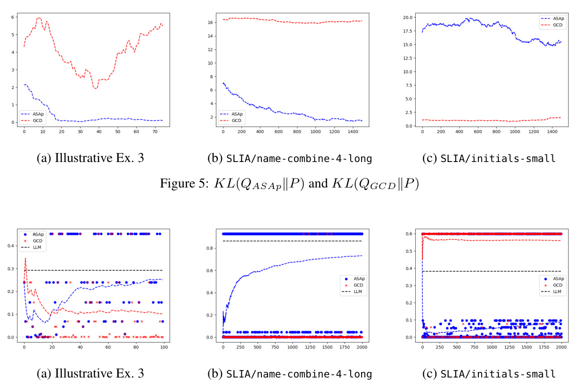
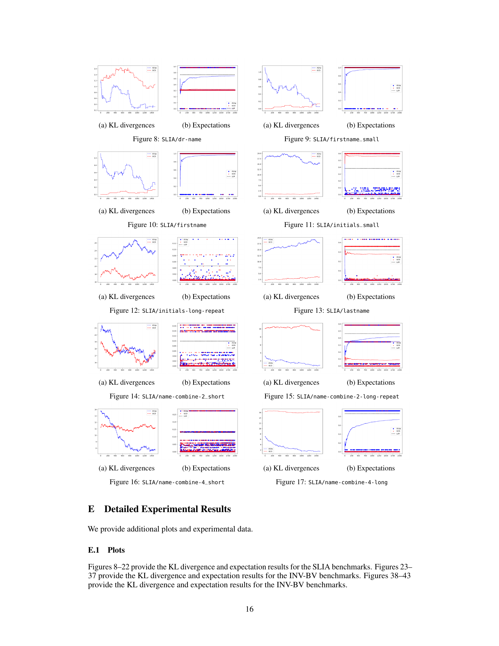
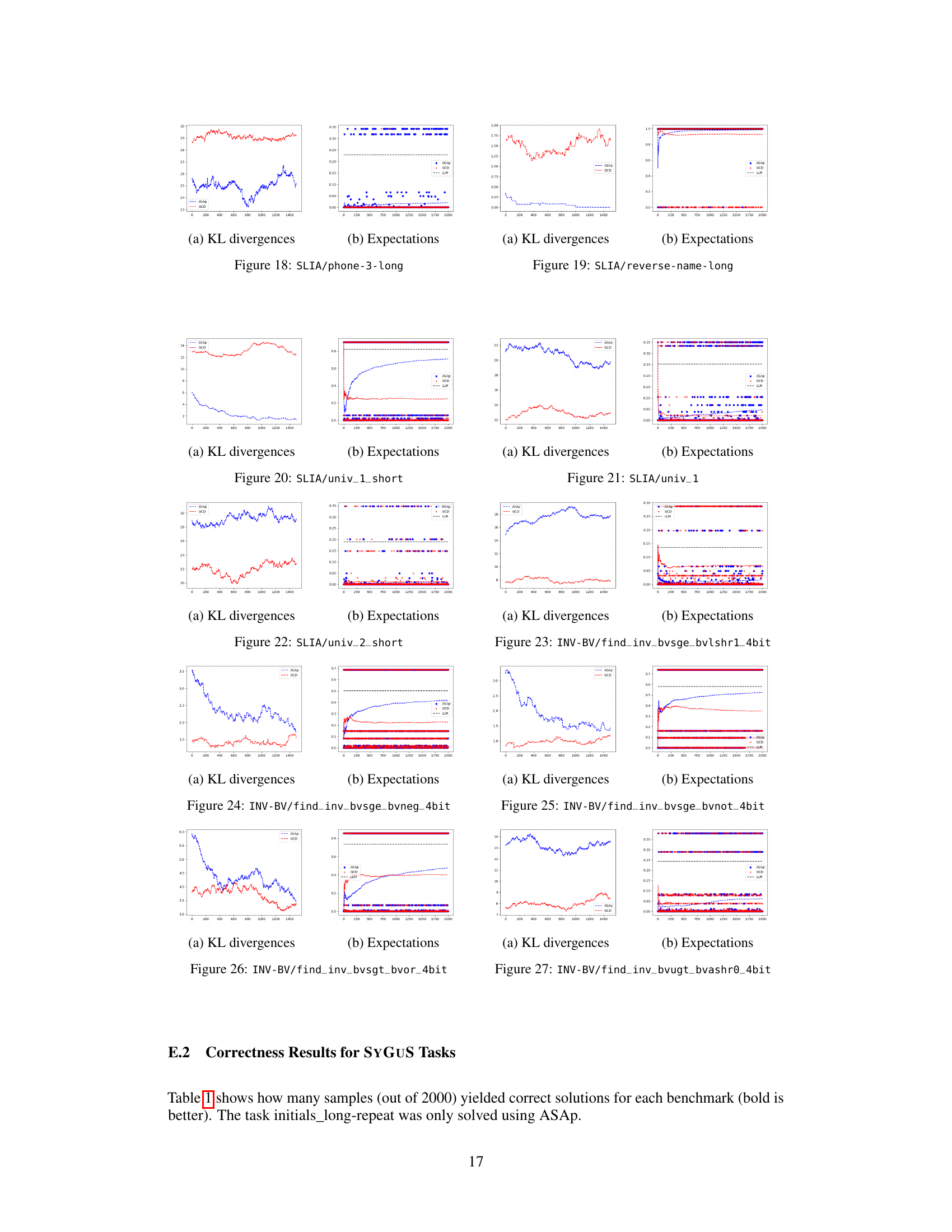
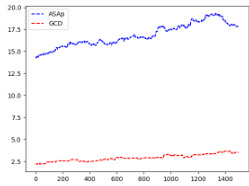
This figure displays the Kullback-Leibler (KL) divergence between the distributions obtained using ASAp (QASAp) and GCD (QGCD) against the original LLM distribution (P) for three different benchmarks: an illustrative example, SLIA/name-combine-4-long, and SLIA/initials-small. The plots show how the KL divergence changes over a certain number of iterations or samples. This illustrates the convergence of ASAp towards the true distribution, which represents the ability of ASAp to align sampling with the grammar constraint without distorting the LLM’s distribution, unlike GCD.

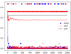
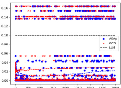
This figure displays scatter plots comparing the empirical expectations of QASAp and QGCD against the true expectation of P (the original LLM distribution) after 2000 samples for three different tasks: SLIA, INV-BV4, and CP. Each point represents a benchmark, with its x-coordinate being the expectation from the LLM distribution and its y-coordinate representing the expectation from either QASAp (blue circles) or QGCD (red crosses). Points close to the diagonal line indicate that the algorithm’s output distribution aligns well with the original LLM distribution, suggesting unbiased sampling.
This figure displays the Kullback-Leibler (KL) divergence between the distributions produced by ASAp and GCD, denoted as QASAp and QGCD respectively, and the original LLM distribution P. The KL divergence is a measure of how different two probability distributions are. Lower KL divergence indicates better alignment with the original distribution. The figure shows KL divergence over a series of iterations for three different benchmarks: (a) Illustrative Ex. 3, (b) SLIA/name-combine-4-long, and (c) SLIA/initials-small. This allows for a visual comparison of how well each algorithm maintains the original LLM distribution while respecting the grammar constraints.

This figure shows the expectations of QASAP, QGCD, and the original LLM distribution P for three different benchmarks: an illustrative example (a), SLIA/name-combine-4-long (b), and SLIA/initials-small (c). Each plot displays the expectation values over time as the number of samples increases, allowing one to observe how the expectations from ASAp and GCD approach or deviate from the true LLM distribution (P). This visual representation helps understand the algorithms’ convergence properties toward the ideal GAD distribution.

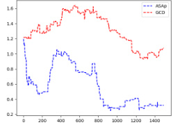
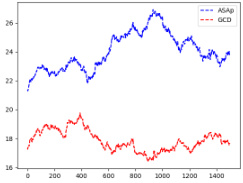
This figure compares the Kullback-Leibler (KL) divergence between the distributions produced by ASAp (QASAp) and GCD (QGCD) and the true distribution P of the language model for three different benchmarks: Illustrative Ex. 3, SLIA/name-combine-4-long, and SLIA/initials-small. The KL divergence is a measure of how different two probability distributions are. A smaller KL divergence indicates a better alignment between the two distributions. The plots show how the KL divergence changes over the number of samples generated. It shows that ASAp’s distribution generally converges more closely to P than GCD’s distribution does.

This figure presents a comparison of the Kullback-Leibler (KL) divergence between the distributions generated by the ASAp and GCD algorithms and the original language model (LLM) distribution (P). The KL divergence measures how different a probability distribution is from a target distribution. A lower KL divergence indicates better alignment. The plots demonstrate the convergence of ASAp and GCD over time. Each subfigure represents a different benchmark task, illustrating the varying convergence speeds and levels of alignment for each method across different tasks.

This figure presents a comparison of the Kullback-Leibler (KL) divergence between the distributions generated by the ASAp and GCD algorithms (QASAp and QGCD, respectively) and the original LLM distribution (P) across multiple benchmarks. The KL divergence serves as a measure of how well the algorithm-generated distributions align with the original LLM distribution, with lower KL values indicating better alignment. The figure visually shows the KL divergence over iterations, allowing for an assessment of convergence and the relative performance of ASAp and GCD. Three subfigures ((a), (b), (c)) show the KL-divergence for different benchmarks: (a) an illustrative example, (b) SLIA/name-combine-4-long benchmark, and (c) SLIA/initials-small benchmark.

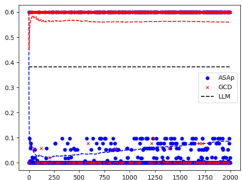
This figure displays the empirical expectations of QASAP, QGCD, and the original language model (P) over 2000 samples for three different benchmarks: an illustrative example (Ex. 3), SLIA/name-combine-4-long, and SLIA/initials-small. The x-axis represents the number of samples, and the y-axis represents the expectation. The plots show how the expectations of QASAP and QGCD converge to the target expectation of P over time. The convergence rate and closeness to the target vary across benchmarks. This is a key visual representation of how ASAp improves over GCD in aligning the sampled distribution with the language model’s distribution, while still respecting the grammatical constraints.

This figure presents a comparison of the Kullback-Leibler (KL) divergence between the distributions generated by ASAp and GCD algorithms, respectively, and the target LLM distribution (P). The KL divergence measures how different the sampled distribution (Q) is from the true distribution of the language model. Lower KL divergence values indicate that the generated distribution is closer to the true distribution of the LLM. The plots show the KL divergence over time (number of samples) for three different benchmarks: Illustrative Ex. 3, SLIA/name-combine-4-long and SLIA/initials-small. It visually shows how ASAp converges faster to the true distribution in all benchmarks, demonstrating that ASAp better aligns with the LLM distribution than GCD.
This figure displays the Kullback-Leibler (KL) divergence between the distributions generated by ASAp and GCD, and the original LLM distribution (P) across iterations. The plots show the KL divergence over time for different tasks. Lower KL divergence indicates better alignment with the original LLM distribution while respecting the grammatical constraints. The plots show that ASAp often converges closer to the target distribution than GCD.
This figure displays the Kullback-Leibler (KL) divergence between the distributions generated by ASAp and GCD and the original LLM distribution (P) for three different benchmarks: Illustrative Ex. 3, SLIA/name-combine-4-long, and SLIA/initials-small. The x-axis represents the number of samples, and the y-axis represents the KL divergence. The plots show how the KL divergence changes as more samples are generated by each algorithm. This helps to visualize the convergence of ASAp and GCD towards the target distribution, illustrating ASAp’s faster convergence and closer alignment with the original LLM distribution.
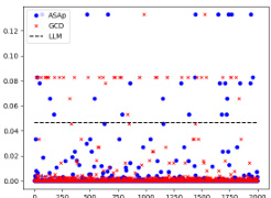
This figure shows scatter plots comparing the empirical expectations of QASAP and QGCD against the expectations of P after 2000 samples for three different tasks: SLIA, INV-BV4, and CP. Each point represents a benchmark, with the x-coordinate being the expectation under P, and the y-coordinate being the expectation under either QASAP or QGCD. Points closer to the diagonal indicate better alignment between the two distributions, suggesting that the sampling methods are accurately reflecting the LLM’s distribution when constrained by the grammar. The plot visually demonstrates the extent to which ASAp better aligns with the expected distribution than GCD, especially for the SLIA and INV-BV4 tasks.
This figure shows the Kullback-Leibler (KL) divergence between the distributions generated by ASAp and GCD and the target distribution P for three different benchmarks: Illustrative Ex. 3, SLIA/name-combine-4-long, and SLIA/initials-small. The KL divergence is a measure of how different two probability distributions are. A lower KL divergence indicates that the two distributions are more similar. In this figure, we can see that ASAp generally achieves a lower KL divergence than GCD, which means that ASAp’s generated distribution is closer to the target distribution than GCD’s. This suggests that ASAp is a better algorithm for grammar-aligned decoding than GCD. The x-axis shows the number of samples and the y-axis shows the KL divergence.
This figure shows the Kullback-Leibler (KL) divergence between the distributions generated by ASAp and GCD, and the target distribution P, for three different benchmarks: an illustrative example from the paper, and two real-world tasks from the SLIA benchmark (name-combine-4-long and initials-small). The x-axis represents the number of iterations, and the y-axis represents the KL divergence. The plots demonstrate how the KL divergence of ASAp converges faster to the ideal distribution P than GCD in the illustrative example and SLIA/name-combine-4-long, while in the SLIA/initials-small benchmark, the convergence is slower but still performs better than GCD.
This figure displays the Kullback-Leibler (KL) divergence between the distributions generated by the ASAp and GCD algorithms and the original LLM distribution (P). The KL divergence measures how different the distributions are. Lower KL divergence indicates better alignment with the original LLM distribution. The figure shows this divergence over multiple iterations (samples) for three different benchmarks: Illustrative Ex. 3, SLIA/name-combine-4-long, and SLIA/initials-small. This helps to visualize the convergence of ASAp towards the LLM’s distribution while adhering to grammatical constraints, whereas GCD shows a larger and more persistent divergence.
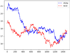
This figure displays the Kullback-Leibler (KL) divergence between the distributions generated by ASAp and GCD (QASAp and QGCD) and the target distribution P. It shows the KL divergence over a series of iterations for three different benchmarks: an illustrative example (a), SLIA/name-combine-4-long (b), and SLIA/initials-small (c). The KL divergence measures how different the generated distributions are from the target LLM distribution, conditioned on the grammar constraints. Lower KL divergence indicates better alignment with the target distribution.
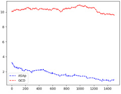
This figure displays the Kullback-Leibler (KL) divergence between the distributions generated by ASAp (approximate grammar-aligned decoding) and GCD (grammar-constrained decoding) and the true distribution P (the original LLM distribution) for three different benchmarks: Illustrative Ex. 3, SLIA/name-combine-4-long, and SLIA/initials-small. The x-axis represents the number of samples, and the y-axis represents the KL divergence. The plots show how quickly the KL divergence between the generated distributions and the true distribution decreases over time. For all the benchmarks, the KL divergence of ASAp decreases faster than that of GCD. This demonstrates that ASAp converges to the LLM distribution much faster than GCD and therefore better preserves the LLM’s distribution when sampling strings that satisfy the constraints of a context-free grammar.
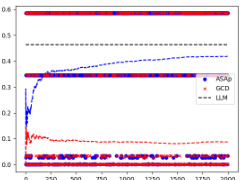
This figure displays the expectation values, or averages, of the probability distributions produced by ASAp, GCD, and the original Language Model (LLM) over the course of 2000 iterations. Each subplot represents a different benchmark task from the paper. The plots visually show how well the sampling distributions of ASAp and GCD align with the LLM’s distribution. The closer the lines are to each other and to the LLM, the better the algorithm is at preserving the LLM’s original distribution while enforcing grammatical constraints.
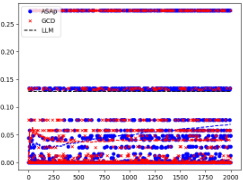
This figure displays the Kullback-Leibler (KL) divergence between the distributions generated by ASAp and GCD, and the target distribution P, across multiple benchmarks. The plots show how quickly the KL divergence of ASAp converges towards zero, which represents alignment with the target distribution. In contrast, GCD’s KL divergence remains higher, indicating a significant distribution mismatch. Three benchmarks, Illustrative Ex. 3, SLIA/name-combine-4-long, and SLIA/initials-small, are shown, highlighting the varying convergence rates across different tasks. This visual representation effectively demonstrates ASAp’s superior performance in producing outputs aligned with the original LLM’s distribution compared to GCD.
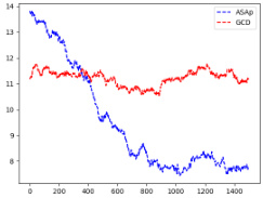
This figure shows the Kullback-Leibler (KL) divergence between the distributions of ASAp and GCD, and the target distribution P for several benchmarks across different numbers of samples. Lower KL divergence indicates better alignment with the target distribution. The plots show that for some benchmarks (e.g., SLIA/name-combine-4-long), ASAp quickly converges to P while GCD does not. For other benchmarks (e.g., SLIA/initials-small), both methods may not converge as quickly, highlighting variations in convergence speeds depending on the task.
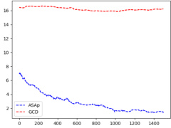
This figure presents KL divergence plots, comparing the distributions generated by ASAp and GCD against the original LLM distribution (P) across various benchmarks. Lower KL divergence indicates a better alignment with the target distribution. It shows how the KL divergence of ASAp decreases over time towards 0, demonstrating its convergence to the LLM’s distribution while respecting grammatical constraints. In contrast, GCD shows less convergence or higher KL divergence, reflecting a greater distortion of the LLM’s distribution.
This figure displays the Kullback-Leibler (KL) divergence between the distributions generated by the ASAp and GCD algorithms and the target LLM distribution (P). The plots show how the KL divergence changes over the number of samples (iterations) for three different tasks: an illustrative example and two tasks from the SLIA benchmark. Lower KL divergence indicates better alignment with the target distribution. The figure shows that ASAp generally converges to the target distribution better than GCD, particularly in the illustrative example and the SLIA/name-combine-4-long benchmark.

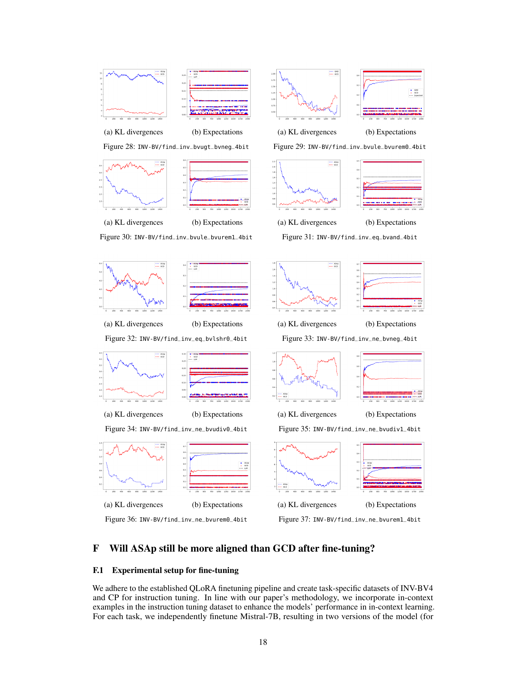
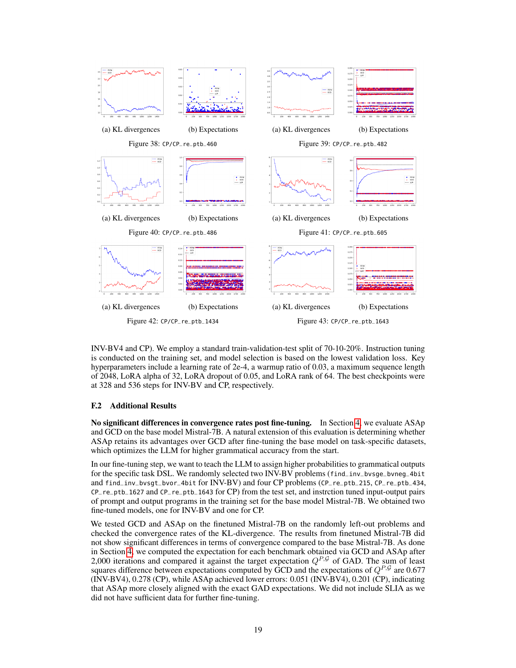
This figure displays the Kullback-Leibler (KL) divergence between the distributions produced by the ASAp and GCD algorithms and the original LLM distribution (P) over 2000 samples. The KL divergence is a measure of how different two probability distributions are. A lower KL divergence indicates that the algorithm’s distribution is closer to the original LLM’s distribution. The figure shows multiple subplots, each representing a different benchmark task. The plots show the KL divergence over time (iterations). Lower values indicate better alignment with the original LLM’s distribution, suggesting higher quality outputs.
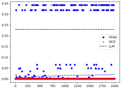
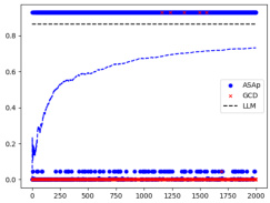
This figure presents a comparison of the performance of ASAp and GCD in matching the expected distribution of the Language Model (LM). Each point represents a benchmark task. The x-coordinate shows the expectation from the LM’s distribution (P), while the y-coordinate shows the empirical expectation obtained using either ASAp or GCD after 2000 sampling iterations. Points close to the diagonal line indicate that the algorithm accurately reflects the LM’s distribution (a good result). The plots reveal that ASAp generally shows better convergence towards the LM’s expectation than GCD, demonstrating ASAp’s effectiveness in aligning the sampling distribution with the desired distribution.

This figure displays the Kullback-Leibler (KL) divergence between the distributions produced by ASAp (QASAp) and GCD (QGCD) and the original LLM distribution (P). The KL divergence measures how different two probability distributions are. A lower KL divergence indicates that the two distributions are more similar. The plots show the KL divergence over the number of samples generated by the algorithms for three different benchmarks: Illustrative Ex. 3, SLIA/name-combine-4-long, and SLIA/initials-small. The plots illustrate how ASAp converges to a distribution that is closer to the LLM’s original distribution than GCD for different structured prediction tasks.
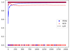
This figure displays the Kullback-Leibler (KL) divergence between the distributions generated by ASAp and GCD (QASAp and QGCD, respectively) and the original LLM distribution (P). The KL divergence measures how different two probability distributions are. A lower KL divergence indicates a closer match between the distributions. The plots show how these divergences change over 2000 iterations/samples for three different benchmarks: an illustrative example and two benchmarks from SLIA (Syntax-Guided Synthesis). The figure helps to visualize the convergence of ASAp’s distribution towards the original LLM distribution.

This figure shows the Kullback-Leibler (KL) divergence between the distributions generated by ASAp and GCD, and the target distribution P. The KL divergence measures how different two probability distributions are. A lower KL divergence indicates that the two distributions are more similar. In this figure, the KL divergence is plotted against the number of samples, allowing us to observe how the algorithms converge to the target distribution over time. The different subfigures correspond to various experiments, each showcasing the convergence behavior of the two algorithms in different structured prediction tasks.
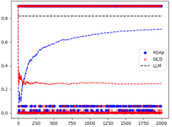
This figure presents the Kullback-Leibler (KL) divergence between the distributions generated by ASAp and GCD, denoted as QASAp and QGCD respectively, and the original LLM distribution P. It shows how the KL divergence changes over the number of samples for three different tasks: an illustrative example (5a), SLIA/name-combine-4-long (5b), and SLIA/initials-small (5c). Lower KL divergence indicates better alignment with the LLM’s original distribution. The plot illustrates that ASAp typically converges to a lower KL divergence than GCD, demonstrating that it better preserves the LLM’s distribution while still enforcing grammatical constraints.
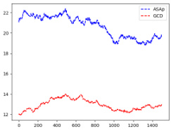
This figure displays the Kullback-Leibler (KL) divergence between the distributions generated by ASAp (QASAp) and GCD (QGCD), and the original LLM distribution (P). The KL divergence is a measure of how different two probability distributions are. Lower KL divergence indicates better alignment between the generated distributions and the original LLM distribution. The figure shows KL divergence over a series of iterations (samples) for three different benchmarks: Illustrative Ex. 3, SLIA/name-combine-4-long, and SLIA/initials-small. The plots illustrate how the KL divergence changes as the number of samples increases for ASAp and GCD on each benchmark, showcasing the convergence properties of each algorithm.

This figure displays the Kullback-Leibler (KL) divergence between the distributions generated by ASAp and GCD, and the original LLM distribution (P). It shows the convergence of KL divergence over 2000 iterations for three different benchmarks: Illustrative Ex. 3, SLIA/name-combine-4-long, and SLIA/initials-small. Lower KL divergence indicates better alignment with the original LLM distribution. The plots reveal that ASAp, in most cases, converges faster and closer to the LLM’s distribution than GCD, indicating that ASAp effectively reduces the distributional distortion caused by constrained decoding.

This figure displays the Kullback-Leibler (KL) divergence between the distributions generated by ASAp and GCD and the target distribution P, plotted against the number of iterations. It shows how ASAp’s KL divergence converges to 0, indicating that it aligns better with the target distribution than GCD. The plots showcase this for three different benchmarks: an illustrative example and two benchmarks from the SLIA dataset.
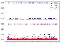
This figure presents scatter plots comparing the empirical expectations obtained using ASAp and GCD against the true expectations from the LLM distribution P, after 2000 sampling iterations. Each point represents a benchmark task. Points closer to the diagonal line (y=x) indicate better alignment between the method’s estimated expectation and the true LLM expectation. The figure visually demonstrates how ASAp, in most cases, achieves a closer alignment to the true LLM expectations compared to GCD.
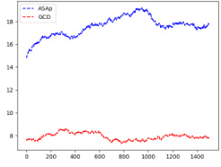
This figure presents a comparison of the Kullback-Leibler (KL) divergence between the distributions generated by ASAp and GCD, respectively, against the target distribution P (the original LLM distribution). The x-axis represents the number of samples, and the y-axis represents the KL divergence. Multiple subfigures show results for different benchmarks, illustrating the convergence behavior of each algorithm in approximating P. Lower KL divergence indicates that the generated distribution is closer to the target distribution, showing better alignment.
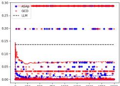
This figure presents a comparison of the empirical expectations obtained using ASAp and GCD against the true expectation from the LLM distribution (P) after 2000 samples. Each point represents a benchmark, with the x-coordinate showing the expectation from P and the y-coordinate showing the expectation from either ASAp or GCD. Points close to the diagonal indicate that ASAp or GCD accurately estimates the LLM’s expectation. The plot helps visualize how close ASAp and GCD get to the true distribution of the LLM, demonstrating ASAp’s superiority in aligning with the target distribution.
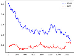
This figure shows the Kullback-Leibler (KL) divergence between the distributions produced by ASAp and GCD, and the original LLM distribution (P). KL divergence is a measure of how different two probability distributions are. Lower KL divergence indicates better alignment with the original LLM distribution. The figure displays KL divergence over a certain number of iterations (samples) for three different benchmarks (Illustrative Ex. 3, SLIA/name-combine-4-long, SLIA/initials-small). It illustrates how ASAp’s distribution aligns more closely with P than GCD’s distribution, especially over more iterations.
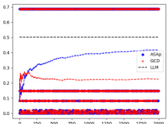
This figure compares the empirical expectations of the variables computed by QASAP and QGCD against the target expectation P for three different benchmarks: Illustrative Ex. 3, SLIA/name-combine-4-long, and SLIA/initials-small. The plots show how the expectations of QASAP and QGCD converge towards the true expectation P over time. In the first benchmark (Illustrative Ex. 3), QASAP quickly converges to P, whereas QGCD does not. The second and third benchmark show varying convergence rates of QASAP towards P and highlight that while QASAP converges towards the correct expectation for all three benchmarks, the rate of convergence varies.
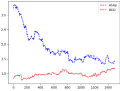
This figure shows the Kullback-Leibler (KL) divergence between the distributions produced by the ASAp and GCD algorithms and the original LLM distribution (P). KL divergence measures how different two probability distributions are; lower values indicate closer agreement. The figure presents results across multiple experiments, showing that ASAp (blue, dashed line) generally demonstrates lower KL divergence than GCD (red, solid line), indicating that ASAp’s output distribution more closely aligns with the LLM’s original distribution while adhering to the grammar constraints.
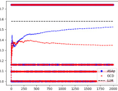
This figure displays the KL divergence between the distributions produced by ASAp and GCD, and the original LLM distribution (P). It visually represents how well the sampling methods align with the true language model distribution, conditioned on the grammatical constraints. Lower KL divergence indicates better alignment. The plots show KL divergence over time (number of samples) for various tasks (Illustrative Ex. 3, SLIA/name-combine-4-long, and SLIA/initials-small), enabling a comparison of ASAp and GCD in terms of their distribution bias.
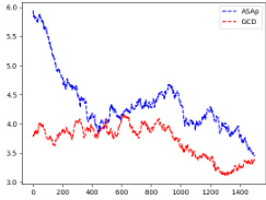
This figure displays KL divergence plots, measuring the difference between the distributions produced by ASAp and GCD and the target LLM distribution (P). It shows the convergence of ASAp and GCD to the LLM distribution over 2000 iterations across various benchmarks: Illustrative Ex. 3, SLIA/name-combine-4-long, and SLIA/initials-small. The plots illustrate how ASAp, in many cases, converges more closely to the LLM’s distribution compared to GCD, indicating that ASAp better preserves the original LLM’s distribution while maintaining grammatical correctness. Note that this is not always the case, depending on the data, as shown in (c).
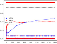
This figure displays the Kullback-Leibler (KL) divergence between the distributions generated by ASAp and GCD, denoted as QASAp and QGCD respectively, and the original LLM distribution P. The KL divergence measures how different the sampled distribution is from the target distribution. Lower KL divergence indicates that the sampled distribution is closer to the target distribution. The figure shows this divergence over 2000 iterations for three different benchmarks. This allows for a visual comparison of the convergence speed and accuracy of both methods in approximating the desired distribution.
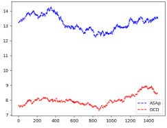
This figure presents a comparison of the Kullback-Leibler (KL) divergence between the distributions generated by ASAp and GCD, and the target distribution P, across multiple benchmarks. Lower KL divergence indicates better alignment with the target distribution. The figure shows that for some benchmarks (e.g., Illustrative Ex. 3 and SLIA/name-combine-4-long), ASAp converges to a lower KL divergence than GCD, demonstrating that it better aligns with the original LLM’s distribution while maintaining grammatical constraints. For other benchmarks (e.g., SLIA/initials-small), the divergence remains high for both algorithms, suggesting that the task might be more challenging.
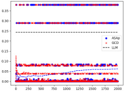
This figure displays the Kullback-Leibler (KL) divergence between the distributions generated by ASAp and GCD, respectively, and the target distribution P over 2000 iterations for three different benchmarks: (a) Illustrative Ex. 3, (b) SLIA/name-combine-4-long, and (c) SLIA/initials-small. The KL divergence measures how different the generated distributions are from the ideal distribution P. Lower KL divergence indicates a better alignment with the target distribution. The plot helps visualize the convergence of the proposed ASAp algorithm towards the desired distribution, as compared to the GCD method.

This figure displays the Kullback-Leibler (KL) divergence between the distributions generated by ASAp (our proposed algorithm) and GCD (existing grammar-constrained decoding), and the target LLM distribution P, across three different benchmarks (Illustrative Ex. 3, SLIA/name-combine-4-long, and SLIA/initials-small). The KL divergence measures how different the generated distributions are from the ideal distribution P. Lower KL divergence indicates better alignment with the original LLM’s distribution, implying higher quality output while preserving grammatical correctness. The plots show KL divergence over the number of samples, illustrating the convergence behavior of the two algorithms.
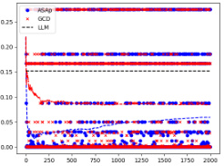
This figure displays the expected values of the probability distributions for QASAP, QGCD, and P. It shows the convergence of ASAp towards the target distribution P across three different benchmarks: Illustrative Example 3, SLIA/name-combine-4-long, and SLIA/initials-small. Each benchmark demonstrates how ASAp’s expectation values approach those of P, indicating the algorithm’s ability to generate samples in line with the original LLM distribution. The figure also illustrates how QGCD is less successful in this regard.
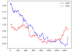
This figure displays the Kullback-Leibler (KL) divergence between the distributions generated by ASAp (QASAp) and GCD (QGCD) and the target distribution P over 2000 iterations for three different benchmarks: Illustrative Ex. 3, SLIA/name-combine-4-long, and SLIA/initials-small. The KL divergence is a measure of how different two probability distributions are. A lower KL divergence indicates that the generated distribution is closer to the target distribution. In all three cases, ASAp demonstrates a lower KL divergence, indicating its superiority to GCD in matching the target distribution.

This figure displays the Kullback-Leibler (KL) divergence between the distributions generated by ASAp and GCD and the target distribution P for three different benchmarks: Illustrative Ex. 3, SLIA/name-combine-4-long, and SLIA/initials-small. The KL divergence is a measure of how different two probability distributions are. A lower KL divergence indicates that the generated distribution is closer to the target distribution. The x-axis represents the number of samples, and the y-axis represents the KL divergence. The figure shows how the KL divergence changes as more samples are generated, giving an indication of convergence to the target distribution. The dashed lines represent the expected KL divergence, highlighting the difference between ASAp and GCD in their approximation of the target distribution.
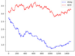
This figure displays the Kullback-Leibler (KL) divergence between the distributions generated by the ASAp and GCD algorithms (QASAp and QGCD, respectively) and the target distribution P (the original LLM distribution) across multiple benchmarks. The KL divergence is a measure of how different two probability distributions are. Lower KL divergence indicates better alignment between the generated and target distributions. The figure visualizes this divergence over many sampling iterations. Three benchmarks are shown, each one demonstrating different convergence speeds. This shows how ASAp, despite starting with a GCD strategy, improves its alignment to P over time.

This figure shows the empirical expectations of QASAP, QGCD, and P for three different benchmarks: Illustrative Ex. 3, SLIA/name-combine-4-long, and SLIA/initials-small. The x-axis represents the number of samples, and the y-axis represents the expectation. The figure demonstrates the convergence of QASAP towards the target distribution P, while QGCD often deviates considerably. Each subplot corresponds to a different benchmark and provides a visual comparison of the expectations from the three methods (ASAP, GCD and P). This helps in visualizing how well the adaptive sampling with approximate expected futures (ASAp) and grammar constrained decoding (GCD) methods approximate the desired probability distribution compared to the true distribution from the language model (P).
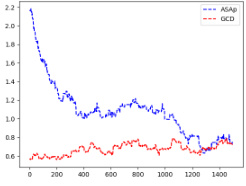
This figure displays the Kullback-Leibler (KL) divergence between the distributions generated by ASAp and GCD, denoted as QASAp and QGCD respectively, compared to the original LLM’s distribution P. The KL divergence is a measure of how different two probability distributions are. Lower values indicate that the distributions are closer, meaning ASAp and GCD are better approximations of P. The figure shows that ASAp’s KL divergence decreases much faster and approaches lower values than GCD’s KL divergence, suggesting that ASAp better preserves the original LLM’s distribution while still ensuring the output is grammatical. Multiple subfigures show results for different benchmarks (Illustrative Ex. 3, SLIA/name-combine-4-long, SLIA/initials-small).
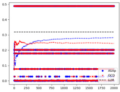
This figure displays the Kullback-Leibler (KL) divergence between the distributions generated by ASAp (QASAp) and GCD (QGCD) compared to the original LLM’s distribution (P). The KL divergence measures how different the sampling distributions of ASAp and GCD are from the true distribution of the language model, conditioned on the grammar. Lower KL divergence indicates better alignment with the LLM’s distribution. The figure shows results for multiple benchmarks, with each subplot representing a different task (‘Illustrative Ex. 3’, ‘SLIA/name-combine-4-long’, and ‘SLIA/initials-small’). The x-axis represents the number of samples, and the y-axis represents the KL divergence.

This figure displays the Kullback-Leibler (KL) divergence between the distributions produced by ASAp and GCD and the target distribution P for three different benchmarks: Illustrative Ex. 3, SLIA/name-combine-4-long, and SLIA/initials-small. The KL divergence measures how different the generated distributions are from the target distribution. A lower KL divergence indicates better alignment with the target. The x-axis represents the number of samples generated, and the y-axis represents the KL divergence. The plots show that ASAp typically converges to a lower KL divergence than GCD, indicating that it produces samples closer to the target distribution.
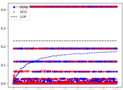
This figure displays the Kullback-Leibler (KL) divergence between the distributions generated by ASAp and GCD and the original LLM distribution (P), for three different benchmarks: Illustrative Ex. 3, SLIA/name-combine-4-long, and SLIA/initials-small. The KL divergence measures how different the generated distributions are from the original LLM distribution. Lower KL divergence indicates better alignment with the original LLM distribution. Each subplot shows the KL divergence over a number of iterations, giving a visual representation of the convergence of both algorithms towards or away from the original distribution. The x-axis represents the number of samples used for the KL divergence calculation, and the y-axis shows the KL divergence value. This allows to see whether either method better respects the LLM distribution while adhering to grammatical constraints.
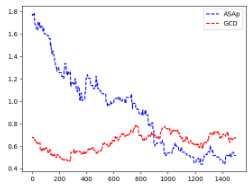
This figure displays the Kullback-Leibler (KL) divergence between the distributions generated by ASAp (QASAp) and GCD (QGCD) and the true distribution P over different iterations. The plots shows the convergence of KL divergence to the target distribution P for three different benchmarks: an illustrative example and two benchmarks from the SLIA task. The y-axis represents the KL divergence, while the x-axis represents the number of iterations. The plots illustrate that ASAp converges more consistently and to a lower KL divergence than GCD across all benchmarks, demonstrating that it better aligns with the true distribution P.
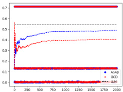
This figure displays the Kullback-Leibler (KL) divergence between the distributions generated by the ASAp and GCD algorithms and the original LLM distribution (P). The KL divergence measures how different the generated distributions are from the original LLM distribution. Lower KL divergence indicates that the generated distribution is closer to the original LLM distribution. The figure shows this divergence for multiple benchmarks (Illustrative Ex. 3, SLIA/name-combine-4-long, and SLIA/initials-small). It shows how the KL divergence changes with the number of samples generated, illustrating the convergence properties of each decoding algorithm. ASAp generally shows better alignment with the LLM’s distribution over time than GCD.
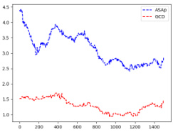
This figure displays the Kullback-Leibler (KL) divergence between the distributions generated by ASAp (QASAp) and GCD (QGCD) and the target distribution P for three different benchmarks: Illustrative Ex. 3, SLIA/name-combine-4-long, and SLIA/initials-small. The KL divergence measures how different the generated distributions are from the ideal distribution. Lower KL divergence indicates a better alignment with the target distribution. The x-axis represents the number of iterations/samples, and the y-axis represents the KL divergence.
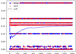
This figure displays the expected values of QASAP, QGCD, and the original LLM distribution P across iterations for three different benchmarks. It demonstrates how the expected values of QASAP converge to those of P over time, indicating the algorithm’s ability to align the sampling distribution with the LLM’s distribution while maintaining grammatical constraints. In contrast, QGCD’s expected values often deviate significantly from P, illustrating how existing constrained decoding methods can distort the LLM’s distribution. The plots show that while in some cases, both ASAp and GCD converge to the same expectation of P, in many cases, ASAp shows closer alignment with P. Therefore, this demonstrates that ASAp is a superior algorithm in cases where high quality of the generated outputs (according to the LLM) are desired.
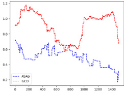
This figure displays the Kullback-Leibler (KL) divergence between the distributions produced by the ASAp and GCD algorithms (QASAp and QGCD, respectively) and the original LLM distribution (P). The KL divergence is a measure of how different two probability distributions are. Lower KL divergence indicates better alignment with the original distribution. The figure shows KL divergence over the number of samples generated, illustrating the convergence properties of ASAp and GCD. Different subfigures represent different tasks or experiments, highlighting how the algorithms perform on various structured prediction problems.
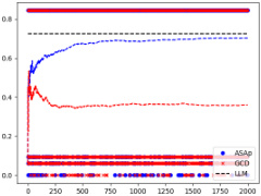
This figure shows the Kullback-Leibler (KL) divergence between the distributions generated by ASAp and GCD from the target distribution P for three different benchmarks (Illustrative Ex. 3, SLIA/name-combine-4-long, and SLIA/initials-small). The KL divergence is a measure of how different two probability distributions are. A lower KL divergence indicates that the two distributions are more similar. In all three benchmarks, ASAp converges to a lower KL divergence than GCD, indicating that ASAp produces outputs that are more similar to the outputs generated by the LLM than GCD. The plots illustrate the convergence of KL divergence over 2,000 iterations or samples.
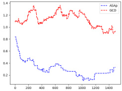
This figure shows the KL divergence between the distributions generated by ASAp and GCD, and the target distribution P, across different numbers of samples. The plots illustrate how the KL divergence changes as the number of samples increases for various benchmarks. Lower KL divergence indicates better alignment with the target distribution, suggesting that ASAp better approximates the target distribution than GCD. The benchmarks used are shown in the subplots.
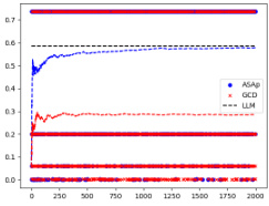
This figure displays the empirical expectation values of QASAP, QGCD, and the original LLM distribution P across different iterations for three benchmarks: an illustrative example and two from the SLIA task (name-combine-4-long and initials-small). The plots show how the expectation values of QASAP converge towards the true expectations given by P, which represents the ideal GAD distribution, while QGCD’s expectations often deviate significantly. This visualization demonstrates the improvement of ASAp over existing methods in aligning the sampling distribution with the desired grammatical constraints.
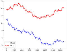
This figure displays the Kullback-Leibler (KL) divergence between the distributions generated by ASAp and GCD (QASAp and QGCD, respectively) and the original LLM distribution (P) across three different tasks: an illustrative example (a), SLIA/name-combine-4-long (b), and SLIA/initials-small (c). The plots show how the KL divergence changes over the number of iterations. Lower KL divergence indicates better alignment between the generated distribution and the original LLM’s distribution, suggesting better preservation of the LLM’s original distribution after applying the constraints. It demonstrates how ASAp better maintains alignment with the original distribution than GCD in each case, although the rate of convergence varies across tasks.
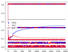
This figure shows the KL divergence between the distributions produced by ASAp and GCD, respectively, and the original LLM distribution P. The plots show how the KL divergence changes over 2000 iterations of sampling for different benchmarks. A lower KL divergence indicates that the algorithm’s output distribution is closer to the original LLM distribution, indicating that ASAp better preserves the LLM’s distribution while ensuring grammaticality.

This figure shows the Kullback-Leibler (KL) divergence between the distributions obtained by ASAp and GCD, and the original LLM distribution (P), for three different benchmarks: Illustrative Ex. 3, SLIA/name-combine-4-long, and SLIA/initials-small. The KL divergence measures how different the distributions are. A lower KL divergence indicates a closer match to the original LLM’s distribution. The plots show the KL divergence over time, allowing comparison of the convergence rates of ASAp and GCD.
Full paper#
