TL;DR#
Recurrent neural networks (RNNs) are powerful but often suffer from instability issues during training, especially in high-dimensional models. Traditional methods use ad-hoc regularization like gradient clipping to address this but lack biological plausibility. Also, neurodynamical models, while biologically realistic, face similar challenges and are notoriously difficult to train.
This paper introduces ORGANICs, a novel recurrent neural circuit model. ORGANICs dynamically implements divisive normalization and leverages the indirect method of Lyapunov to prove its remarkable unconditional local stability for high-dimensional models. This intrinsic stability allows for training without gradient clipping. Empirical results demonstrate that ORGANICs outperforms other neurodynamical models on image classification and performs comparably to LSTMs on sequential tasks, showcasing its efficacy and potential.
Key Takeaways#
Why does it matter?#
This paper is crucial for researchers in neural networks and neuroscience because it introduces ORGANICs, a novel recurrent neural circuit model that is both biologically plausible and effortlessly trainable. Its unconditional stability eliminates the need for ad hoc regularization techniques, thereby advancing both theoretical understanding and practical applications of recurrent neural networks. Furthermore, it opens avenues for developing more interpretable and robust deep learning models inspired by biological principles.
Visual Insights#
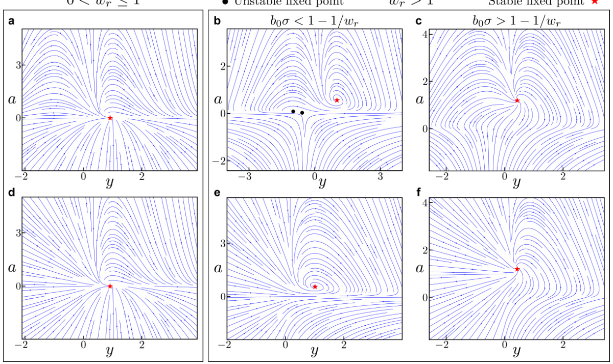
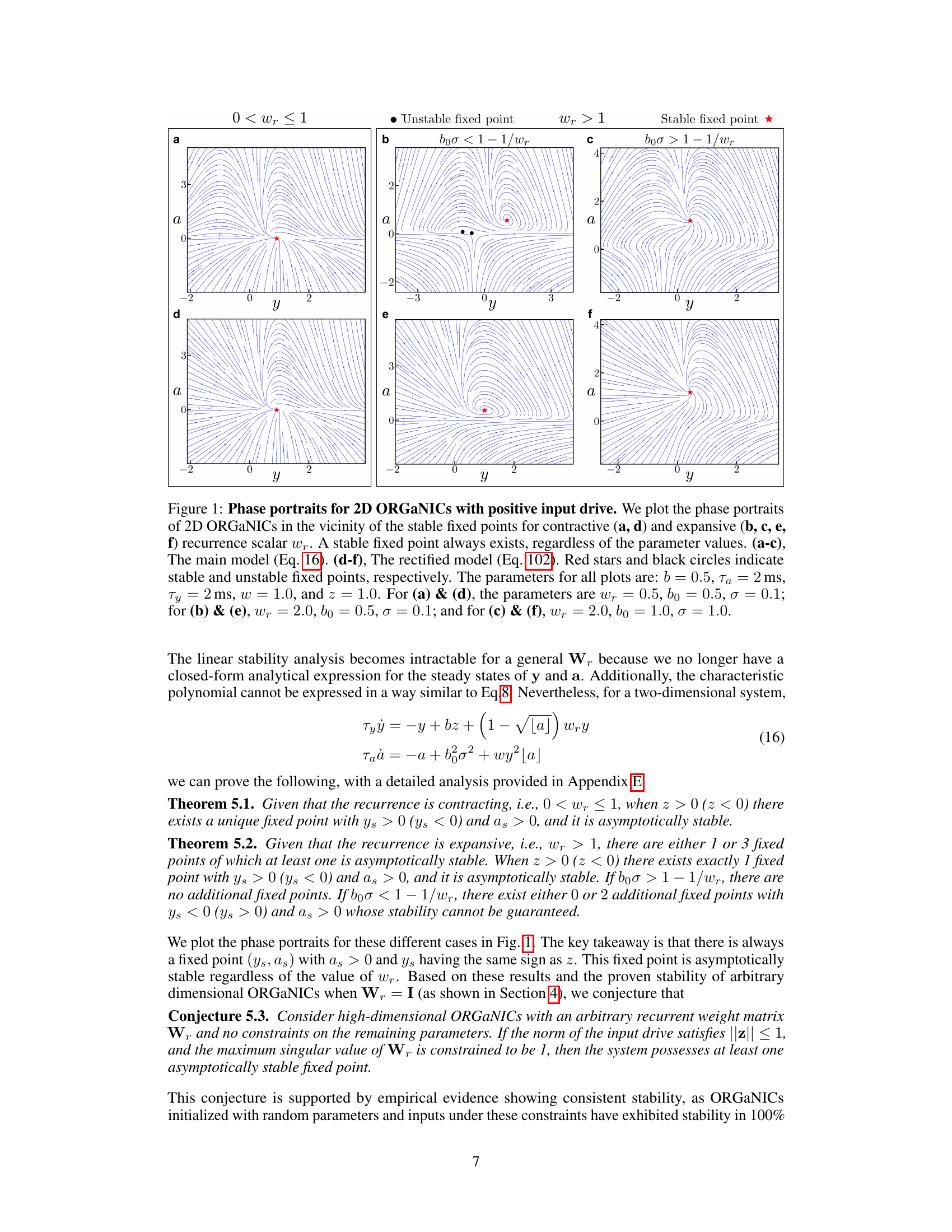
🔼 This figure displays phase portraits of a two-dimensional ORGANICs model. It shows how the system’s behavior changes with different recurrence strengths (wr) and input drives (z). The plots illustrate that a stable fixed point always exists in both contractive (wr<1) and expansive (wr>1) regimes, showing the robustness of the model.
read the caption
Figure 1: Phase portraits for 2D ORGANICs with positive input drive. We plot the phase portraits of 2D ORGANICs in the vicinity of the stable fixed points for contractive (a, d) and expansive (b, c, e, f) recurrence scalar wr. A stable fixed point always exists, regardless of the parameter values. (a-c), The main model (Eq. 16). (d-f), The rectified model (Eq. 102). Red stars and black circles indicate stable and unstable fixed points, respectively. The parameters for all plots are: b = 0.5, τα = 2ms, Ty = 2ms, w = 1.0, and z = 1.0. For (a) & (d), the parameters are wr = 0.5, bo = 0.5, σ = 0.1; for (b) & (e), wr = 2.0, bo = 0.5, σ = 0.1; and for (c) & (f), wr = 2.0, bo = 1.0, σ = 1.0.
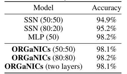
🔼 This table presents the test accuracy results of different models on the MNIST handwritten digit classification task. The models compared include Stabilized Supralinear Networks (SSNs) with different configurations (50:50 and 80:20 representing the ratio of excitatory to inhibitory neurons), a Multilayer Perceptron (MLP), and the proposed Oscillatory Recurrent Gated Neural Integrator Circuits (ORGANICs) model with different configurations and a two-layer version. The table demonstrates that ORGANICs achieves comparable or superior performance to the other models on this task.
read the caption
Table 1: Test accuracy on MNIST dataset
In-depth insights#
DN & Stability#
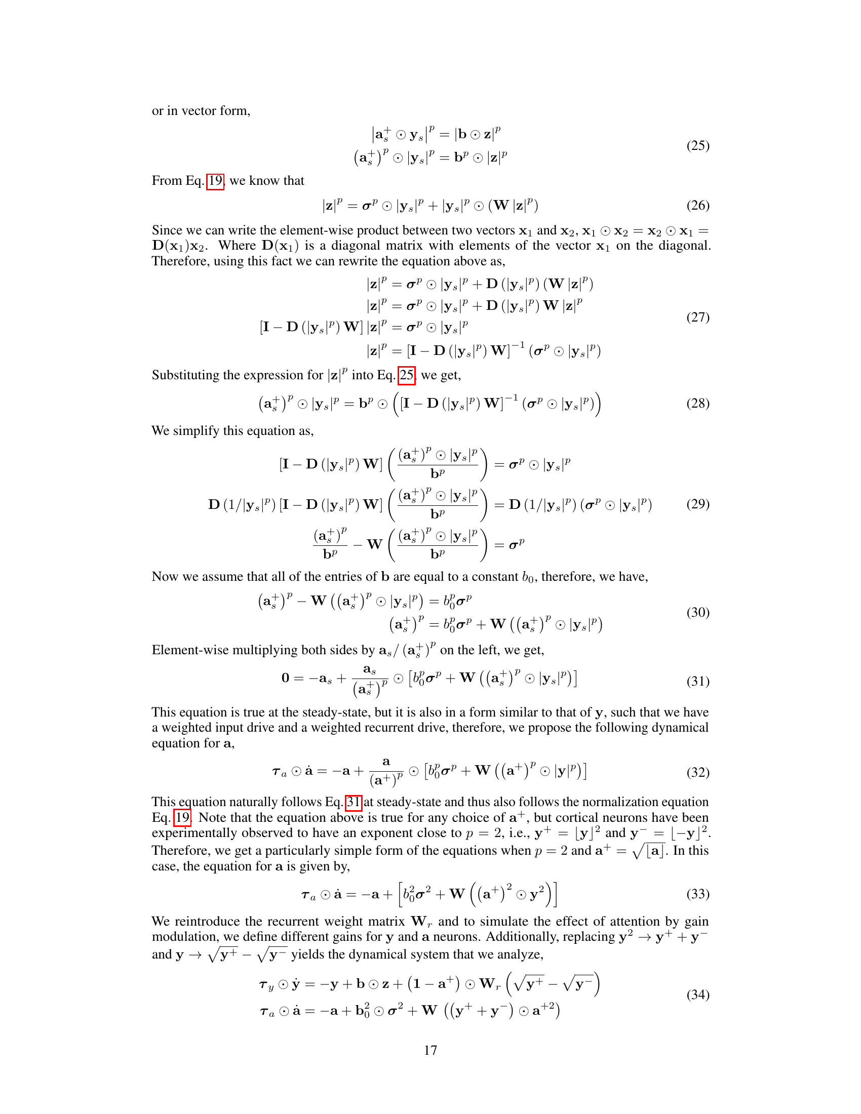
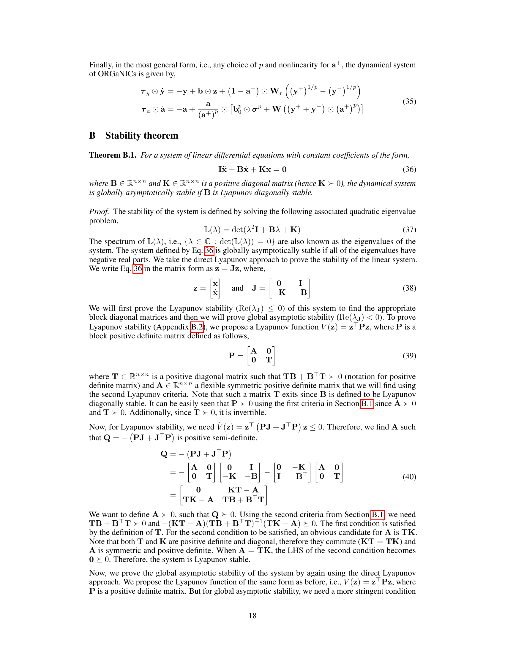
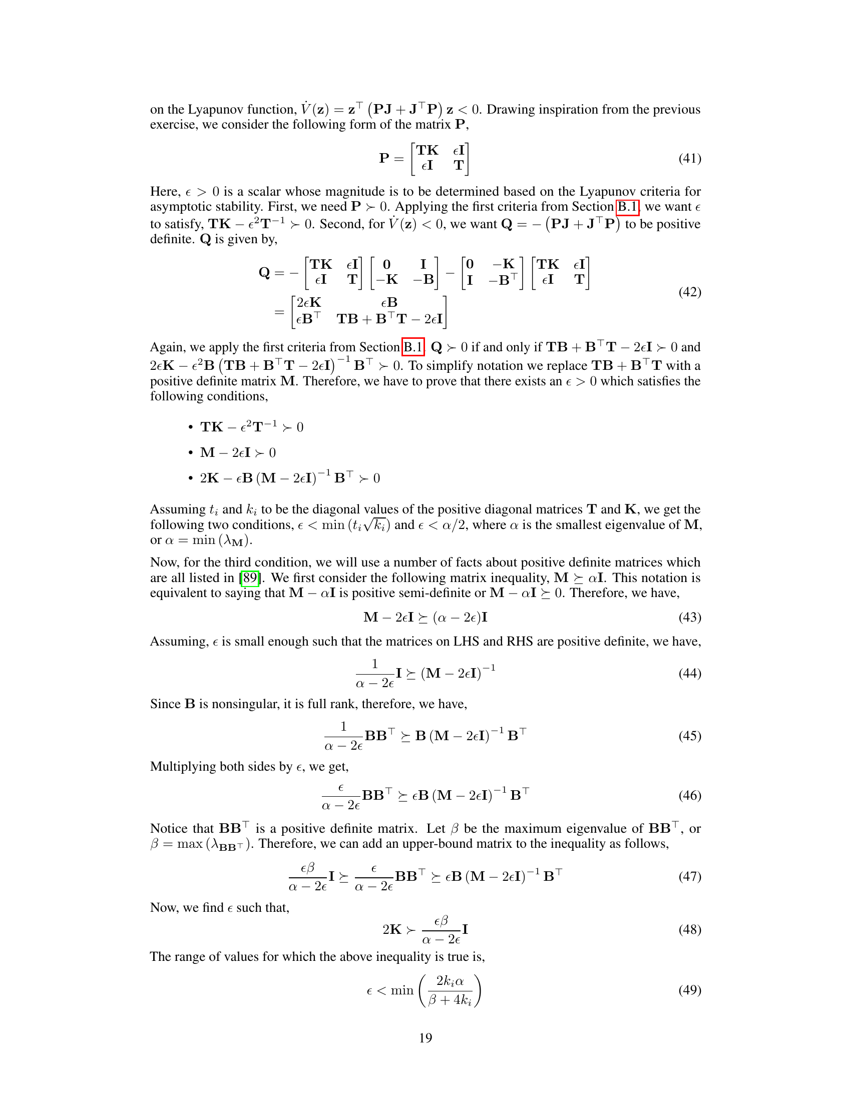
The research explores the relationship between divisive normalization (DN) and the stability of recurrent neural networks (RNNs), particularly focusing on a biologically plausible model called ORGANICs. DN, a fundamental neural computation, is shown to be intrinsically linked to the stability of ORGANICs. The authors demonstrate that under specific conditions (such as an identity recurrent weight matrix), ORGANICs exhibit unconditional local stability. This stability is mathematically proven using the indirect method of Lyapunov, connecting the circuit’s dynamics to a system of coupled damped harmonic oscillators. Importantly, this inherent stability allows for seamless training of ORGANICs through backpropagation through time without the need for gradient clipping or scaling, unlike many other RNN models. The research further investigates the stability of ORGANICs with more generic weight matrices, offering both theoretical analysis and empirical evidence supporting the claim of robust stability. This connection between DN and stability is a significant contribution, highlighting the potential of biologically-inspired designs for building more stable and trainable neural networks.
ORGANICs Model#
The ORGANICs (Oscillatory Recurrent Gated Neural Integrator Circuits) model is a biologically plausible recurrent neural network architecture designed to dynamically implement divisive normalization (DN). Its key innovation lies in directly incorporating DN into its recurrent dynamics, rather than adding it as a post-processing step. This leads to several advantages. Firstly, ORGANICs exhibit unconditional local stability under specific conditions, making them significantly easier to train than traditional RNNs which often suffer from exploding or vanishing gradients. Secondly, the inherent stability allows for training via standard backpropagation-through-time (BPTT) without the need for gradient clipping or other ad-hoc regularization techniques. This simplifies the training process and enhances biological plausibility. Thirdly, the model’s steady-state response adheres to the DN equation, linking its behavior directly to well-established neurobiological phenomena and enhancing interpretability. The connection between DN and stability is a major contribution, offering a principled way to build more stable and biologically realistic RNNs.
BPTT Training#
Backpropagation through time (BPTT) is a crucial training method for recurrent neural networks (RNNs), enabling the learning of temporal dependencies in sequential data. However, training RNNs with BPTT often faces challenges like exploding and vanishing gradients, hindering convergence and performance. This paper introduces ORGANICs, a biologically plausible recurrent neural circuit model that dynamically implements divisive normalization (DN). A key finding is that ORGANICs’ inherent stability, stemming from DN, allows for robust BPTT training without the need for gradient clipping or other regularization techniques. This is a significant advantage over traditional RNNs, which frequently require such ad hoc methods to mitigate instability issues. The empirical results demonstrate that ORGANICs, trained via straightforward BPTT, achieves performance comparable to LSTMs on sequence modeling tasks, showcasing the effectiveness and efficiency of its intrinsic stability in the context of BPTT training.
RNN Benchmarks#
RNN benchmarks are crucial for evaluating the performance of recurrent neural networks, especially when comparing novel architectures like the ORGANICs model discussed in the research paper. A comprehensive benchmark suite should include tasks assessing diverse aspects of RNN capabilities: long-short-term memory (LSTM) tasks, requiring handling of long-range dependencies in sequential data; tasks emphasizing complex temporal dynamics, such as those found in video processing or natural language understanding; and static input tasks, demonstrating the network’s ability to process non-sequential data. The choice of benchmark datasets is critical; well-established datasets like Penn Treebank or IMDB reviews for language modeling, and CIFAR-10 or ImageNet for image processing tasks, offer standardized evaluations. Performance metrics beyond simple accuracy, like perplexity for language, precision/recall for classification, or even computational efficiency, should be reported. ORGANICS would benefit from a comparison with state-of-the-art RNNs across these various benchmarks to highlight its strengths and weaknesses in a fair and nuanced evaluation.
Future Works#
The “Future Works” section of this research paper envisions several promising avenues. A key area is exploring multi-layer ORGANICs architectures with feedback connections, mirroring the complex structure of the cortex. This will allow assessment of performance on more sophisticated sequential modeling tasks and cognitive problems involving long-term dependencies. Another critical area is investigating how the model’s intrinsic time constants can be modulated, enabling the model to learn and adapt to various time scales, and effectively functioning as a flexible working memory system. The authors also plan to explore the application of more compact or convolutional weight matrices to scale the model more effectively to higher dimensions, addressing a current limitation. Finally, a deeper investigation into the biological plausibility of ORGANICs is proposed, by relating model parameters and dynamics to specific neurophysiological mechanisms.
More visual insights#
More on figures
🔼 This figure shows phase portraits of a two-dimensional ORGANICs model with positive input drive, illustrating the stability of the model for both contractive and expansive recurrence. It displays how the system converges to a stable fixed point under various parameter settings, regardless of the choice of recurrence weight (wr).
read the caption
Figure 1: Phase portraits for 2D ORGANICs with positive input drive. We plot the phase portraits of 2D ORGANICs in the vicinity of the stable fixed points for contractive (a, d) and expansive (b, c, e, f) recurrence scalar wr. A stable fixed point always exists, regardless of the parameter values. (a-c), The main model (Eq. 16). (d-f), The rectified model (Eq. 102). Red stars and black circles indicate stable and unstable fixed points, respectively. The parameters for all plots are: b = 0.5, τα = 2ms, Ty = 2ms, w = 1.0, and z = 1.0. For (a) & (d), the parameters are wr = 0.5, bo = 0.5, σ = 0.1; for (b) & (e), wr = 2.0, bo = 0.5, σ = 0.1; and for (c) & (f), wr = 2.0, bo = 1.0, σ = 1.0.
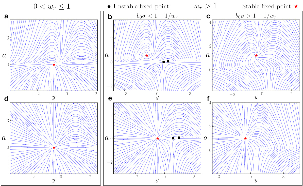
🔼 This figure shows phase portraits of a two-dimensional ORGANICs model for both contractive and expansive recurrence. It demonstrates the existence of a stable fixed point regardless of the parameter values, highlighting the robustness of the model.
read the caption
Figure 1: Phase portraits for 2D ORGANICs with positive input drive. We plot the phase portraits of 2D ORGANICs in the vicinity of the stable fixed points for contractive (a, d) and expansive (b, c, e, f) recurrence scalar wr. A stable fixed point always exists, regardless of the parameter values. (a-c), The main model (Eq. 16). (d-f), The rectified model (Eq. 102). Red stars and black circles indicate stable and unstable fixed points, respectively. The parameters for all plots are: b = 0.5, τα = 2ms, Ty = 2ms, w = 1.0, and z = 1.0. For (a) & (d), the parameters are wr = 0.5, bo = 0.5, σ = 0.1; for (b) & (e), wr = 2.0, bo = 0.5, σ = 0.1; and for (c) & (f), wr = 2.0, bo = 1.0, σ = 1.0.

🔼 This figure shows phase portraits of the 2D rectified ORGANICs model for three different sets of time constants: Ty = Ta, Ty < Ta, and Ty > Ta. Each plot displays the dynamics of the system in the phase plane (y, a), with the stable fixed points marked by red stars. The figure demonstrates how changing the ratio of time constants (Ty/Ta) affects the dynamics and stability of the system.
read the caption
Figure 3: Phase portraits for 2D rectified ORGANICs for different time constants. Red stars indicate stable fixed points. The parameters for all plots are: w₁ = 1.0, bo = 0.5, b = 0.5, σ = 0.1, w = 1.0, and z = 1.0. For (a), the time constants are Ta = 2ms, Ty = 2ms; for (b), Ta = 10 ms, Ty = 2 ms; for (c), Ta = 2ms, Ty = 10 ms.
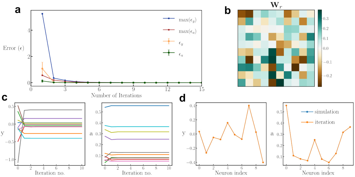
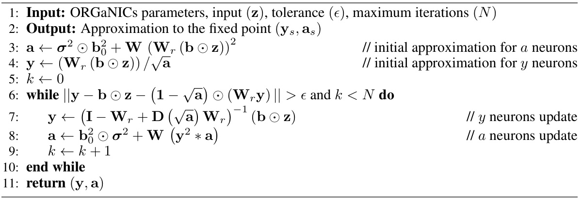
🔼 This figure demonstrates the fast convergence of an iterative algorithm used to find the fixed point of a 20-dimensional ORGANICS model. It shows that the algorithm quickly converges to the true solution, even when starting from random initial conditions. The figure includes plots showing error convergence, a sample weight matrix, the iterative process for several neurons, and the overlap between the iterative and true solutions.
read the caption
Figure 4: Fast convergence of the iterative algorithm. The results are for 20-dimensional ORGANICS (10 y and 10 a neurons) with random parameters and inputs with the additional constraint of the maximum singular value of Wr equal to 1 and ||z|| < 1. (a), Mean (with error bars representing 1-sigma S.D.) and maximum errors (€) as a function of number of iterations. e is calculated as the norm of the difference between the true solution (found by simulation starting with random initialization) and the iteration solution. (b), An example of a randomly sampled Wr. (c), Steady-state approximation as a function of iteration number. Different lines represent different neurons. (d), Overlap between the iteration solution (after 15 iterations) and the true solution.
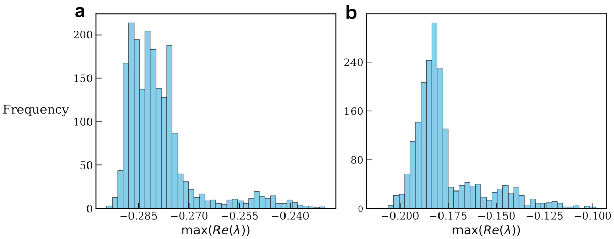
🔼 This figure shows the histograms of the real part of the eigenvalues with the largest real part for a two-layer ORGANICS model trained on the static MNIST classification task. The model’s recurrent weight matrix (Wr) was constrained to have a maximum singular value of 1. The histograms demonstrate that all eigenvalues have negative real parts, indicating asymptotic stability in both layers. The separate histograms for each layer highlight the independent stability analysis possible due to the feedforward structure of the model.
read the caption
Figure 5: Histogram for the eigenvalue with the largest real part. We train two-layer ORGANICS (Ta = Ty = 2ms) with a static MNIST input where Wr is constrained to have a maximum singular value of 1. We plot the histogram of eigenvalues of the Jacobian matrix with the largest real part, for inputs from the test set. We find that all the eigenvalues of the Jacobian have negative real parts, implying asymptotic stability. (a), histogram for the first layer. (b), histogram for the second layer. Note that since this is implemented in a feedforward manner, this is a cascading system with no feedback, hence we can perform the stability analysis of the two layers independently.

🔼 The figure shows the largest real part of eigenvalues across all test samples as training progresses for a static MNIST classification task. The fact that the largest real part consistently remains below zero indicates that the system maintains stability throughout the training process.
read the caption
Figure 6: Eigenvalue with the largest real part while training on static input (MNIST) classification task. This plot shows the largest real part of eigenvalues across all test samples as training progresses. The fact that the largest real part consistently remains below zero indicates that the system maintains stability throughout training.
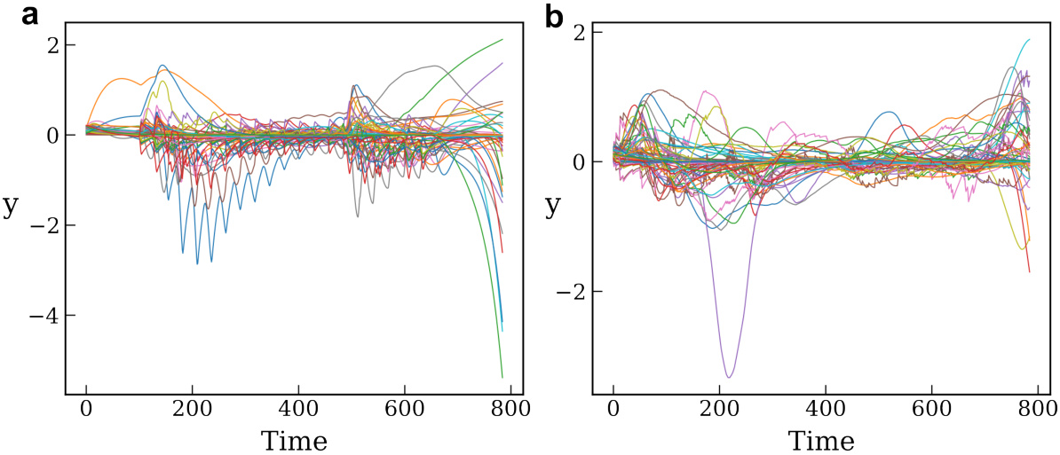
🔼 This figure shows the bounded trajectories of the hidden states (y) of ORGANICs neural network trained as RNN on unpermuted and permuted sequential MNIST datasets. The plots demonstrate the stability of the network by showing that the hidden state values remain within a limited range during the sequential input presentation.
read the caption
Figure 7: Trajectories of the hidden states (y). This plot shows the dynamics of the hidden state as the input is being presented sequentially. We train ORGANICs (128 units) as an RNN on (a), unpermuted sequential MNIST and (b), permuted sequential MNIST. The inputs are picked randomly from the test set. The hidden state trajectory remains bounded, indicating stability.
More on tables
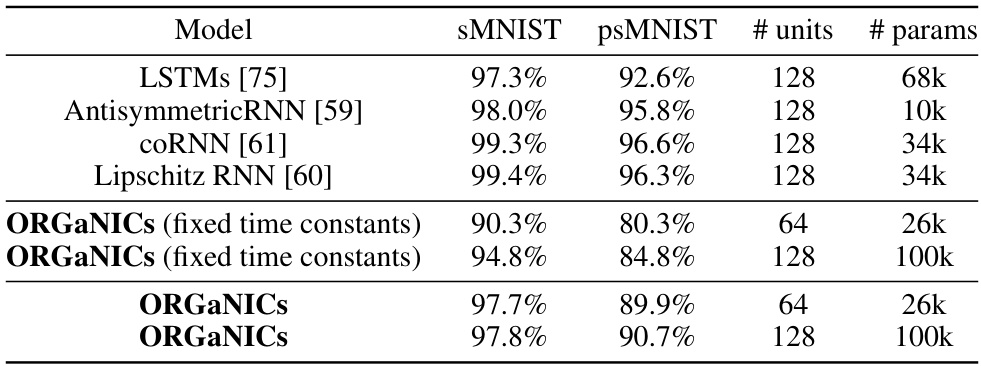
🔼 This table compares the performance of ORGANICs against other RNN models on two sequential MNIST tasks: the standard sequential MNIST (sMNIST) and the permuted sequential MNIST (psMNIST). The sMNIST task involves classifying MNIST digits from their pixels presented sequentially in scanline order. psMNIST adds a further challenge by randomly permuting the pixel order before presentation. The table shows the test accuracy, the number of hidden units, and the number of parameters for each model. ORGANICs achieves performance comparable to LSTMs on sMNIST and only slightly lower on psMNIST, even without using ad-hoc techniques like gradient clipping.
read the caption
Table 2: Test accuracy on sequential pixel-by-pixel MNIST and permuted MNIST

🔼 This table details the parameterization used for the ORGANICs model in the static MNIST classification task. It specifies whether each parameter (Wzx, Wbx, Wr, W, bo, σ) is learned during training or fixed, its shape (dimensions), and its initialization method. The parameters represent different aspects of the model, including input weights, recurrent weights, normalization weights, input gains, and normalization constants.
read the caption
Table 4: ORGANICs parametrization for static MNIST classification
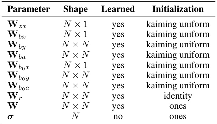
🔼 This table lists the parameters used in the ORGANICs model for static MNIST classification, their shapes, whether they are learned during training, and their initialization methods. The parameters include weight matrices for input (Wzx, Wbx), recurrent connections (Wby, Wba), input gain modulation (Wbox, Wboy, Wboa), the recurrent weight matrix (Wr), normalization weights (W), and the parameters σ for divisive normalization. The initialization methods include kaiming uniform and identity matrix.
read the caption
Table 4: ORGANICs parametrization for static MNIST classification

🔼 This table shows the hyperparameters used for training the ORGANICs model on the static and sequential MNIST image classification tasks. For the static MNIST task, there was no step size for the learning rate scheduler. In contrast, for the sequential MNIST task, the step size for the learning rate scheduler was set to 30 epochs and the gamma to 0.8.
read the caption
Table 7: Hyperparameters
Full paper#
