TL;DR#
Language models have rapidly advanced, but understanding the drivers of this progress is crucial. Previous research focused on hardware improvements, following Moore’s Law. However, this overlooks the significant influence of algorithmic innovation and improvements in model training techniques. This paper addresses this gap by analyzing the interplay of these factors to determine what has truly fueled the recent advancements.
The researchers developed augmented scaling laws to disentangle the contributions of algorithms and compute scaling. They compiled a dataset of over 200 language model evaluations to perform this analysis, revealing that compute scaling has been the more dominant factor in recent years. However, they also highlight the importance of algorithmic progress, particularly from the introduction of the Transformer architecture, which has drastically improved efficiency. Their analysis provides a nuanced perspective on AI progress, offering a more comprehensive understanding of the factors driving its rapid advancements and guiding future research and development.
Key Takeaways#
Why does it matter?#
This paper is crucial for researchers in AI and related fields as it quantifies the rapid progress in language modeling, separating the contributions of compute scaling from algorithmic advancements. This provides valuable insights for future research directions, policy decisions, and resource allocation.
Visual Insights#

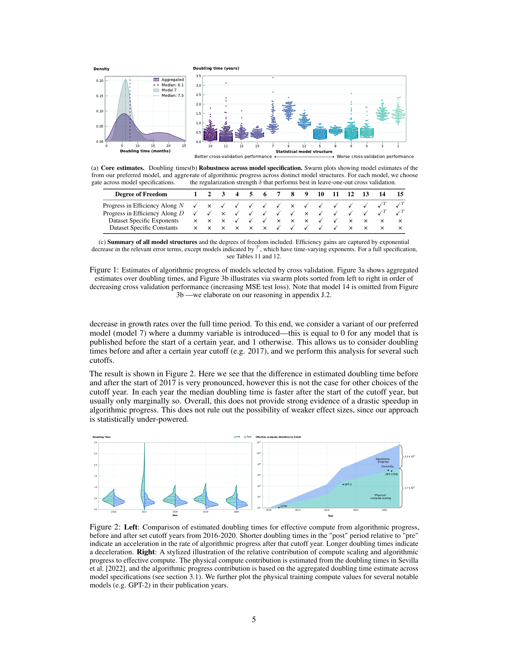
🔼 This figure presents the findings of cross-validation exercises to determine the best-fitting model for estimating algorithmic progress. Figure 1a shows a density plot of the doubling times (in months) estimated by the preferred model and an aggregate of many models, revealing a median doubling time around 7-8 months. Figure 1b displays swarm plots illustrating model estimates of the rate of algorithmic progress across various model structures; models performing better in cross-validation are on the left, with doubling times decreasing as cross-validation performance improves. The omission of model 14 is discussed in the appendix.
read the caption
Figure 1: Estimates of algorithmic progress of models selected by cross validation. Figure 3a shows aggregated estimates over doubling times, and Figure 3b illustrates via swarm plots sorted from left to right in order of decreasing cross validation performance (increasing MSE test loss). Note that model 14 is omitted from Figure 3b-we elaborate on our reasoning in appendix J.2.

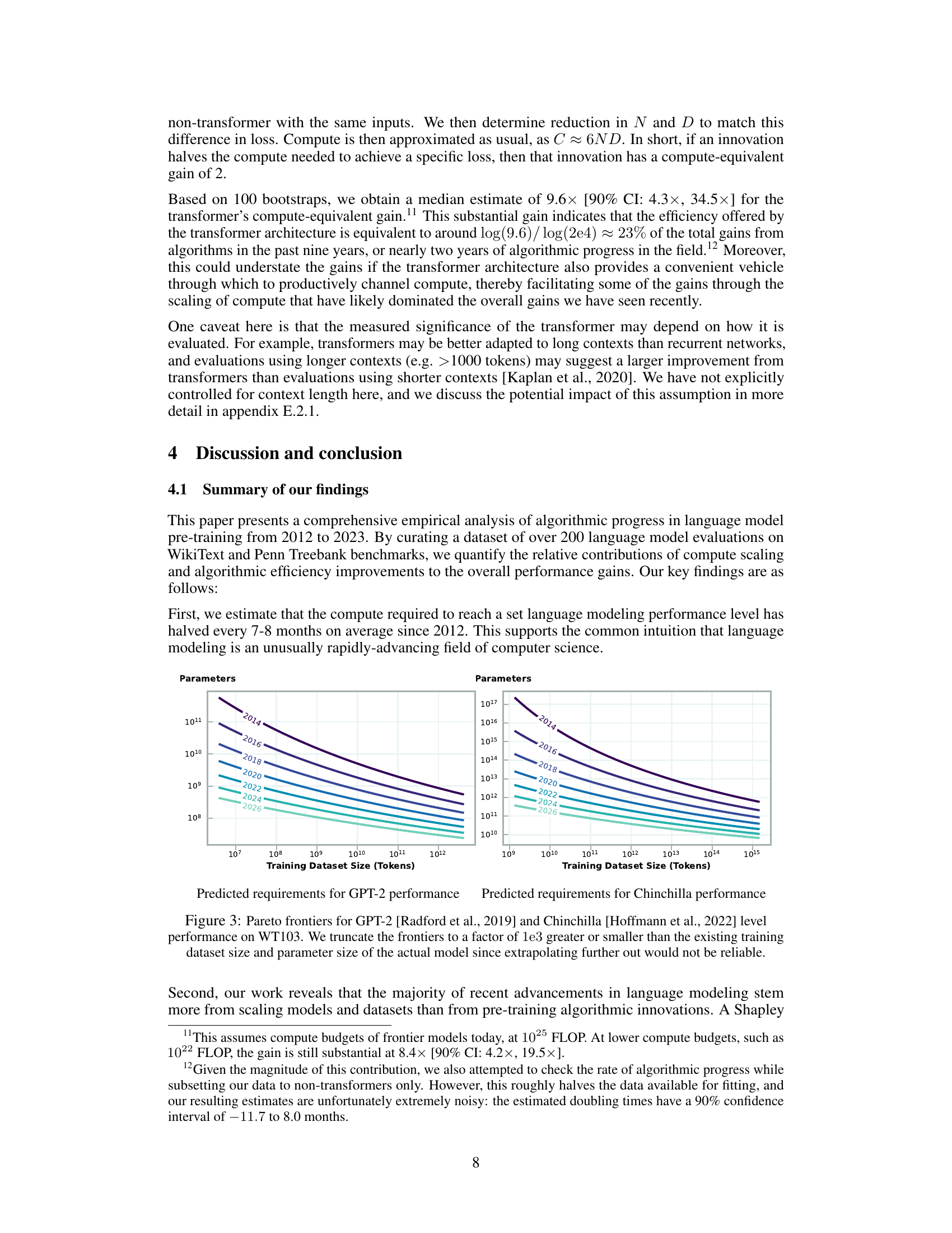
🔼 This table shows the Shapley decomposition of progress in pre-training language models between pairs of models. It breaks down the contributions of algorithmic improvements and compute scaling to the overall performance gains between each model pair. Note that the Shapley values are based on point estimates and are for illustration only, and parameter efficiency is omitted due to its insignificance. The table focuses on the earliest decoder-only transformer model in the dataset.
read the caption
Table 1: Attribution of progress to pre-training algorithmic progress and compute scaling between model pairs based on Shapley decomposition in linear space. Numbers may not all add up to 100% due to rounding. These Shapley values are based on point estimates from our preferred model and as such are meant for illustrative purposes only. We omit parameter efficiency improvements from the table since these are almost always 0% and not very informative. The Transformer here is by Baevski and Auli [2018] (the earliest decoder-only transformer we have in our dataset), who modify the original transformer architecture by Vaswani et al. [2017] to be decoder-only.
In-depth insights#
Algorithmic Progress Rate#
Analyzing the rate of algorithmic progress is crucial for understanding the trajectory of artificial intelligence. The paper investigates this by examining the compute required to achieve specific performance thresholds in language models over time. A key finding is the surprisingly rapid pace of this progress, significantly outpacing Moore’s Law. This suggests that algorithmic innovations, not just hardware improvements, are major drivers of enhanced capabilities. The study also attempts to quantify the relative contribution of increased compute versus algorithmic improvements. While compute scaling plays a larger role overall, the paper highlights that algorithmic breakthroughs like the transformer architecture have made significant independent contributions. Further research is needed to fully disentangle the roles of these factors and to better predict future algorithmic advances. The analysis, while insightful, is subject to limitations including noisy benchmark data and the difficulty of isolating the impact of individual algorithmic innovations. Nevertheless, it provides valuable evidence about the rapid evolution of this field and its multifaceted drivers.
Scaling Laws’ Impact#
The impact of scaling laws on large language models (LLMs) is profound. Scaling laws have empirically demonstrated a strong correlation between model size, dataset size, and compute resources, and the resulting performance. This suggests a predictable path towards improved model capabilities, driven by increasing these factors. However, simple extrapolation of scaling laws has limitations. Algorithmic advancements play a critical, albeit less easily quantified role, and their contribution may change over time as model scales increase. The relationship between compute scaling and algorithmic progress is complex and intertwined; algorithmic innovations can significantly improve the efficiency of compute usage, but compute scaling itself remains a dominant driver of performance improvements. Furthermore, the scale-dependence of algorithmic progress introduces challenges in predicting future model capabilities. Certain algorithmic improvements may be more effective at larger scales, while others might become less relevant. Therefore, a nuanced understanding of scaling laws is crucial, recognizing both their predictive power and limitations, to effectively guide future research and development in the field of LLMs.
Transformer’s Role#
The transformer architecture’s emergence revolutionized language modeling. Its parallel processing capability, unlike recurrent networks, drastically reduced training time and enabled scaling to unprecedented sizes. This efficiency boost was a pivotal factor in the rapid progress observed, contributing significantly more than incremental algorithmic improvements. While the paper quantifies the overall impact of compute scaling over algorithmic advancements, the transformer’s unique contribution deserves further detailed investigation. Its impact is more than just a faster training time; it enabled entirely new model sizes and architectures which in themselves drive further performance gains. The study touches on this, showing a substantial ‘compute-equivalent gain’, highlighting the transformative nature of the architecture. Future research should delve into the nuances of the transformer’s impact, considering its role in enabling new scaling laws and the interplay between architectural innovation and the scaling of computational resources. This deeper understanding is crucial for predicting future progress in the field.
Methodology Limits#
Limitations in methodology significantly impact the reliability and generalizability of research findings. Data limitations, such as noise, sparsity, and inconsistencies in evaluation metrics across studies, introduce uncertainty into any conclusions. Model selection challenges in choosing appropriate statistical models to capture diverse phenomena within a dataset also contribute to potential biases. The paper’s reliance on specific scaling laws may restrict the applicability of its conclusions beyond those specific modeling techniques. Extrapolations, extending the observed trends to future AI developments, lack direct empirical support, increasing the likelihood of inaccurate predictions. Overall, a thorough acknowledgment of these methodological constraints is crucial for a balanced interpretation of the results. The reliance on extrapolation highlights a need for further, direct evidence to validate the long-term trends inferred from the study.
Future Research#
Future research directions stemming from this paper could explore several key areas. Firstly, a more granular analysis of algorithmic progress is needed, moving beyond broad trends to pinpoint specific innovations and their relative contributions. This could involve examining changes in specific model architectures, training techniques, or data preprocessing methods over time. Secondly, the impact of data quality and dataset composition on algorithmic gains requires further study. Benchmark datasets are not static; evolution in tokenization and data preprocessing will influence apparent progress. Thirdly, a deeper investigation into the interaction between algorithmic improvements and scaling laws is essential. Current models assume a simple multiplicative relationship, yet the interplay likely exhibits more nuance. Finally, understanding the limitations of extrapolating current trends into the future is crucial. While the compute-driven acceleration observed is striking, its sustainability and the emergence of novel algorithmic paradigms remain open questions.
More visual insights#
More on figures

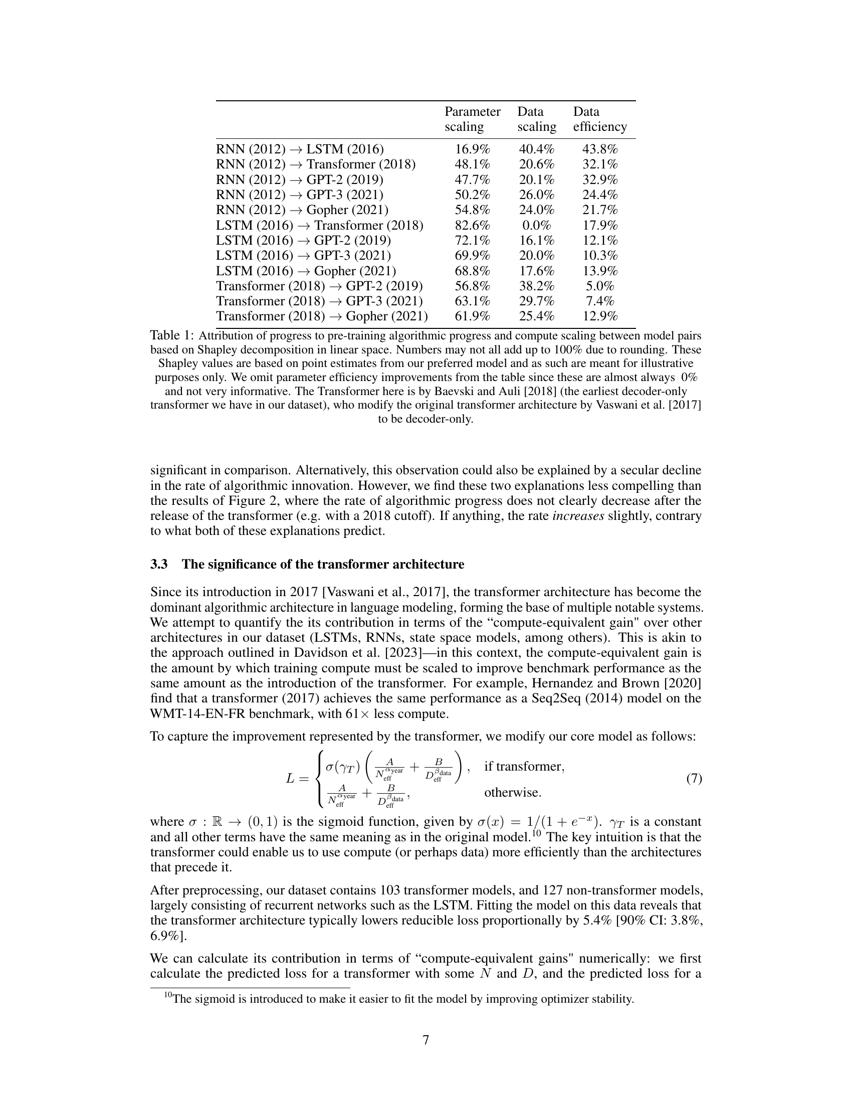
🔼 The left panel shows the estimated doubling times for effective compute from algorithmic progress before and after different cutoff years (2016-2020). Shorter doubling times after the cutoff year suggest an acceleration in algorithmic progress, while longer doubling times imply deceleration. The right panel visualizes the relative contributions of compute scaling and algorithmic progress to the overall growth of effective compute, using data from Sevilla et al. (2022) and the aggregated doubling time estimate from the paper. The plot also includes the physical training compute values for some notable language models.
read the caption
Figure 2: Left: Comparison of estimated doubling times for effective compute from algorithmic progress, before and after set cutoff years from 2016–2020. Shorter doubling times in the “post” period relative to “pre” indicate an acceleration in the rate of algorithmic progress after that cutoff year. Longer doubling times indicate a deceleration. Right: A stylized illustration of the relative contribution of compute scaling and algorithmic progress to effective compute. The physical compute contribution is estimated from the doubling times in Sevilla et al. [2022], and the algorithmic progress contribution is based on the aggregated doubling time estimate across model specifications (see section 3.1). We further plot the physical training compute values for several notable models (e.g., GPT-2) in their publication years.

🔼 Figure 3 presents the analysis of doubling times in algorithmic progress for language models, based on model selection using cross-validation. Subfigure (a) shows the aggregated estimates of doubling times, while subfigure (b) provides swarm plots showing the distribution of doubling time estimates across different model structures, sorted by their cross-validation performance (in increasing mean squared error). Note that Model 14 is excluded from subfigure (b), with explanations provided in Appendix J.2.
read the caption
Figure 3: Estimates of algorithmic progress of models selected by cross validation. Figure 3a shows aggregated estimates over doubling times, and Figure 3b illustrates via swarm plots sorted from left to right in order of decreasing cross validation performance (increasing MSE test loss). Note that model 14 is omitted from Figure 3b-we elaborate on our reasoning in appendix J.2.
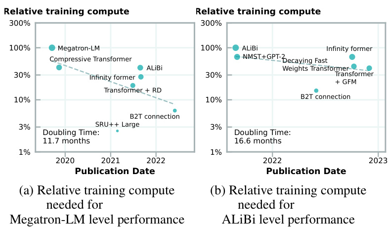
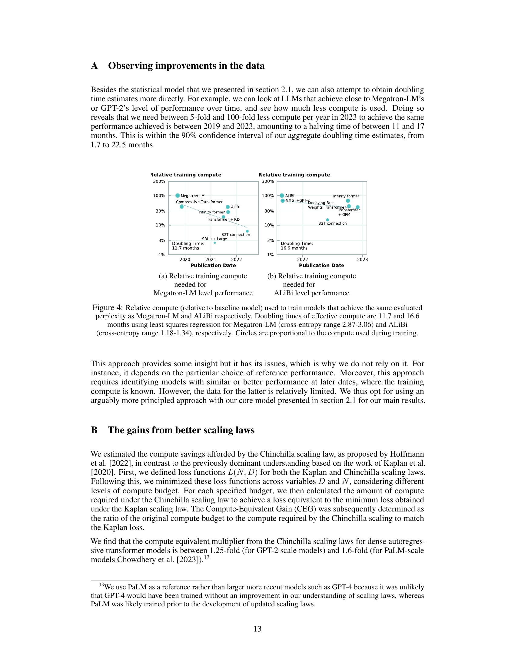
🔼 This figure shows the relative compute needed to achieve the same perplexity as Megatron-LM and ALiBi models over time. The left panel shows that to match Megatron-LM’s performance, the compute needed has halved approximately every 11.7 months. The right panel shows a similar trend for ALiBi, with compute halving roughly every 16.6 months. The size of the circles reflects the compute used during training.
read the caption
Figure 4: Relative compute (relative to baseline model) used to train models that achieve the same evaluated perplexity as Megatron-LM and ALiBi respectively. Doubling times of effective compute are 11.7 and 16.6 months using least squares regression for Megatron-LM (cross-entropy range 2.87-3.06) and ALiBi (cross-entropy range 1.18-1.34), respectively. Circles are proportional to the compute used during training.

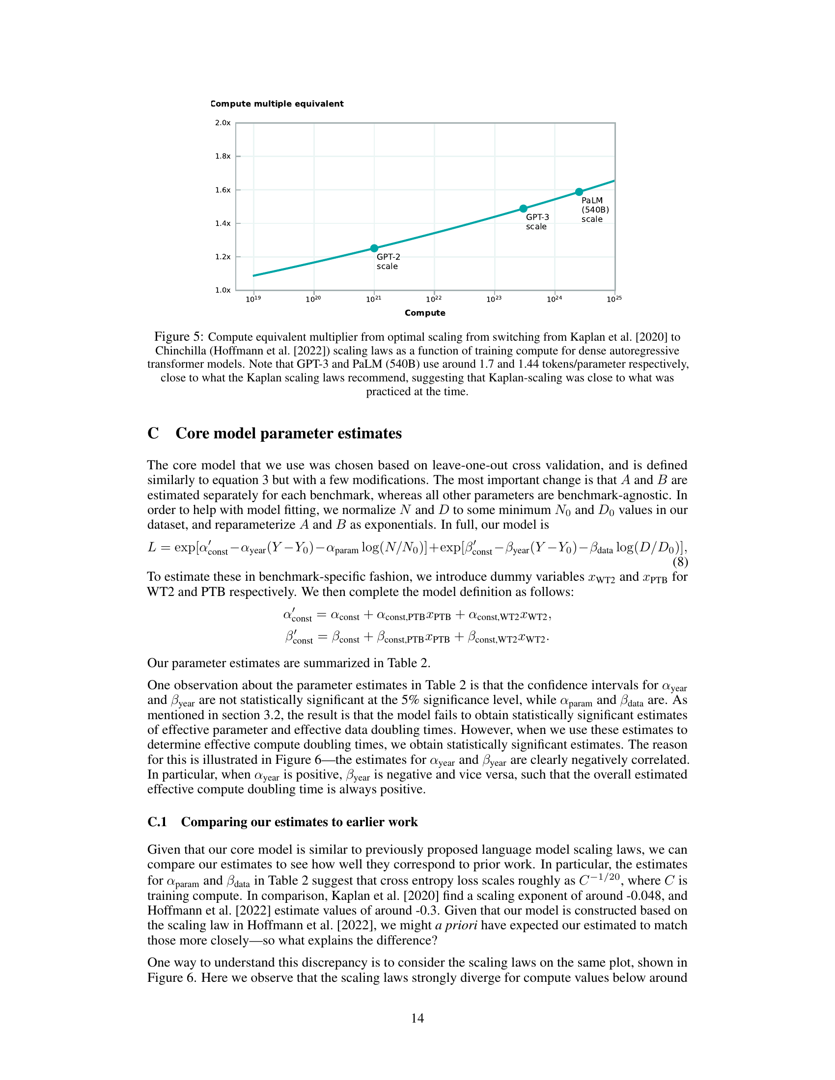
🔼 This figure shows the compute-equivalent gain obtained from switching from Kaplan et al.’s scaling law to Chinchilla’s scaling law. The x-axis represents the training compute, and the y-axis shows the compute-equivalent multiplier. It shows that the compute-equivalent gain increases as the training compute increases, and that GPT-3 and PaLM models already used parameter-to-token ratios that were close to the optimal values suggested by Kaplan et al.
read the caption
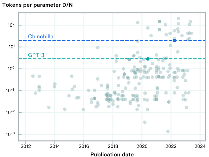
Figure 5: Compute equivalent multiplier from optimal scaling from switching from Kaplan et al. [2020] to Chinchilla (Hoffmann et al. [2022]) scaling laws as a function of training compute for dense autoregressive transformer models. Note that GPT-3 and PaLM (540B) use around 1.7 and 1.44 tokens/parameter respectively, close to what the Kaplan scaling laws recommend, suggesting that Kaplan-scaling was close to what was practiced at the time.
🔼 This figure presents the results of cross-validation analysis for different model structures used to estimate the rate of algorithmic progress in language models. Panel (a) shows the distribution of doubling time estimates from the preferred model and aggregated estimates across all models. Panel (b) uses swarm plots to illustrate the model estimates for different model structures, ordered by cross-validation performance (from best to worst). Note that model 14 is excluded from (b), with the reason explained in Appendix J.2.
read the caption
Figure 1: Estimates of algorithmic progress of models selected by cross validation. Figure 3a shows aggregated estimates over doubling times, and Figure 3b illustrates via swarm plots sorted from left to right in order of decreasing cross validation performance (increasing MSE test loss). Note that model 14 is omitted from Figure 3b-we elaborate on our reasoning in appendix J.2.

🔼 This figure shows the results of cross-validation for different models used to estimate algorithmic progress. Figure 1a presents a density plot of doubling times for effective compute, comparing the core estimates from the preferred model and the aggregation of all considered models. Figure 1b uses swarm plots to show the robustness of the doubling time estimates across various model specifications, ordered by cross-validation performance. Figure 1c summarizes the different model structures and degrees of freedom. The core analysis focuses on the doubling time of compute and data efficiency improvements due to algorithmic progress in pre-training.
read the caption
Figure 1: Estimates of algorithmic progress of models selected by cross validation. Figure 3a shows aggregated estimates over doubling times, and Figure 3b illustrates via swarm plots sorted from left to right in order of decreasing cross validation performance (increasing MSE test loss). Note that model 14 is omitted from Figure 3b-we elaborate on our reasoning in appendix J.2.
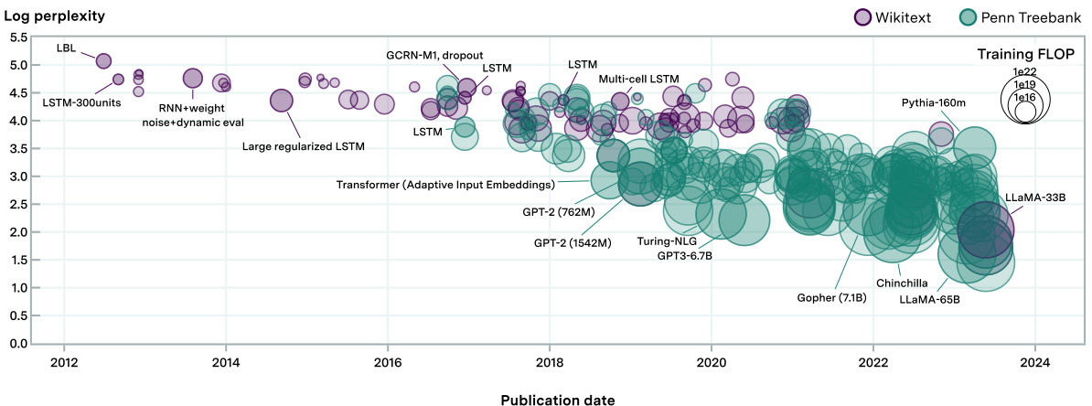
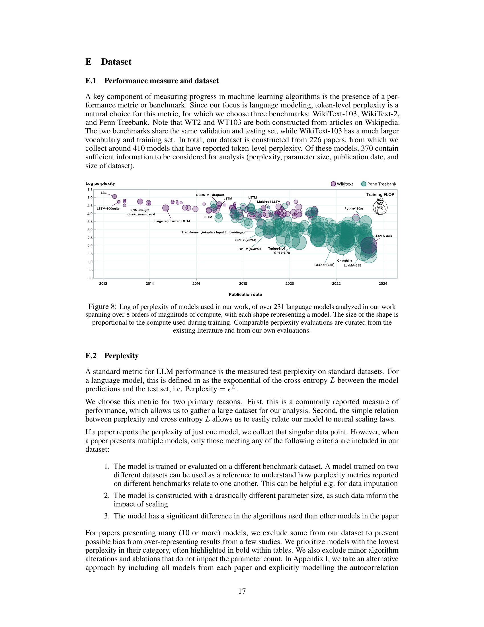
🔼 This figure shows the log perplexity of over 231 language models plotted against their publication date. The size of each point corresponds to the amount of compute used in training that model. The models are categorized by whether they were evaluated on WikiText or Penn Treebank. The plot visually demonstrates the rapid decrease in perplexity (improvement in performance) and the massive increase in compute used over time.
read the caption
Figure 8: Log of perplexity of models used in our work, of over 231 language models analyzed in our work spanning over 8 orders of magnitude of compute, with each shape representing a model. The size of the shape is proportional to the compute used during training. Comparable perplexity evaluations are curated from the existing literature and from our own evaluations.

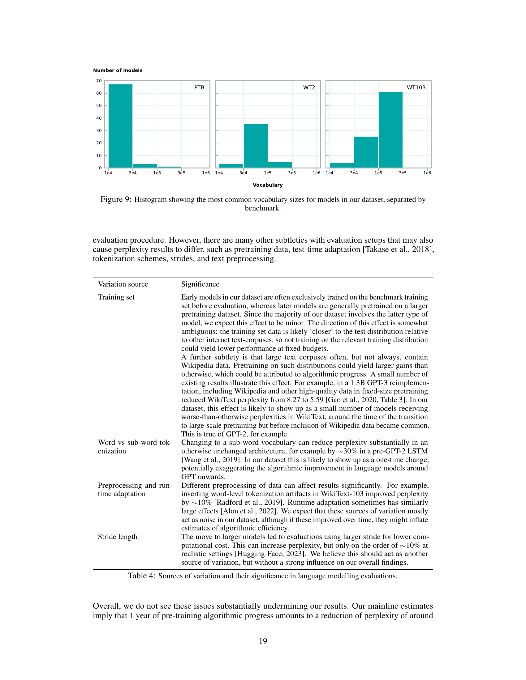
🔼 This figure shows the distribution of vocabulary sizes across the three benchmarks used in the study: PTB, WT2, and WT103. The x-axis represents the vocabulary size, and the y-axis represents the number of models. The figure helps to visualize the concentration of models around certain vocabulary sizes within each benchmark. It highlights the prevalence of certain vocabulary size ranges within each dataset used for the language modeling experiments.
read the caption
Figure 9: Histogram showing the most common vocabulary sizes for models in our dataset, separated by benchmark.
🔼 The left panel shows the estimated doubling times for effective compute before and after different cutoff years. The shorter doubling times in the period after the cutoff year indicate an acceleration in the rate of algorithmic progress. Conversely, the longer doubling times suggest a deceleration. The right panel shows a stylized illustration of how compute scaling and algorithmic progress contribute to the effective compute. The physical compute contribution is estimated from the doubling time found by Sevilla et al (2022). The contribution from algorithmic progress is based on the aggregated doubling times obtained across various model specifications, which are explained in section 3.1 of the paper. The figure also includes the physical training compute values for some notable models at the time of their publication.
read the caption
Figure 2: Left: Comparison of estimated doubling times for effective compute from algorithmic progress, before and after set cutoff years from 2016–2020. Shorter doubling times in the 'post' period relative to 'pre' indicate an acceleration in the rate of algorithmic progress after that cutoff year. Longer doubling times indicate a deceleration. Right: A stylized illustration of the relative contribution of compute scaling and algorithmic progress to effective compute. The physical compute contribution is estimated from the doubling times in Sevilla et al. [2022], and the algorithmic progress contribution is based on the aggregated doubling time estimate across model specifications (see section 3.1). We further plot the physical training compute values for several notable models (e.g., GPT-2) in their publication years.

🔼 This figure presents the results of the cross-validation analysis used to select the best statistical model for estimating the rate of algorithmic progress. Panel (a) shows the distribution of doubling time estimates from the preferred model and from an aggregation across all models considered. Panel (b) displays a swarm plot showing the doubling time estimates for various model structures sorted from best to worst cross-validation performance. Model 14 is excluded from this plot for reasons detailed in Appendix J.2.
read the caption
Figure 1: Estimates of algorithmic progress of models selected by cross validation. Figure 3a shows aggregated estimates over doubling times, and Figure 3b illustrates via swarm plots sorted from left to right in order of decreasing cross validation performance (increasing MSE test loss). Note that model 14 is omitted from Figure 3b-we elaborate on our reasoning in appendix J.2.
More on tables

🔼 This table shows the decomposition of progress in language models between pairs of models into the contributions of algorithmic progress and compute scaling using the Shapley value decomposition method. The table focuses on the relative contributions of these two factors and omits parameter efficiency due to its negligible contribution.
read the caption
Table 1: Attribution of progress to pre-training algorithmic progress and compute scaling between model pairs based on Shapley decomposition in linear space. Numbers may not all add up to 100% due to rounding. These Shapley values are based on point estimates from our preferred model and as such are meant for illustrative purposes only. We omit parameter efficiency improvements from the table since these are almost always 0% and not very informative. The Transformer here is by Baevski and Auli [2018] (the earliest decoder-only transformer we have in our dataset), who modify the original transformer architecture by Vaswani et al. [2017] to be decoder-only.
🔼 This table shows the decomposition of progress into pre-training algorithmic progress and compute scaling for different model pairs. The Shapley value decomposition method is used to quantify the relative contributions of each factor. Note that parameter efficiency improvements are omitted due to their consistently negligible values. The table uses the earliest decoder-only transformer model available in the dataset as a reference point for comparison.
read the caption
Table 1: Attribution of progress to pre-training algorithmic progress and compute scaling between model pairs based on Shapley decomposition in linear space. Numbers may not all add up to 100% due to rounding. These Shapley values are based on point estimates from our preferred model and as such are meant for illustrative purposes only. We omit parameter efficiency improvements from the table since these are almost always 0% and not very informative. The Transformer here is by Baevski and Auli [2018] (the earliest decoder-only transformer we have in our dataset), who modify the original transformer architecture by Vaswani et al. [2017] to be decoder-only.
🔼 This table presents the results of a Shapley value decomposition analysis of the relative contributions of pre-training algorithmic progress and compute scaling to performance improvements between pairs of language models. It shows the percentage contribution of each factor for various model pairs, highlighting the increasing importance of compute scaling over time. Note that some values may not sum to 100% due to rounding.
read the caption
Table 1: Attribution of progress to pre-training algorithmic progress and compute scaling between model pairs based on Shapley decomposition in linear space. Numbers may not all add up to 100% due to rounding. These Shapley values are based on point estimates from our preferred model and as such are meant for illustrative purposes only. We omit parameter efficiency improvements from the table since these are almost always 0% and not very informative. The Transformer here is by Baevski and Auli [2018] (the earliest decoder-only transformer we have in our dataset), who modify the original transformer architecture by Vaswani et al. [2017] to be decoder-only.
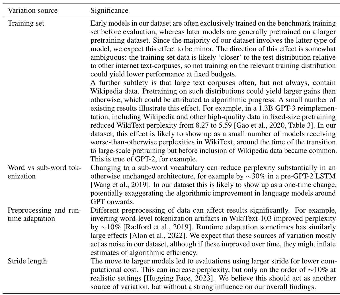
🔼 This table presents the results of a Shapley value decomposition analysis showing the relative contributions of algorithmic progress and compute scaling to the improvements in language model performance between different pairs of models. The analysis decomposes the progress into percentage contributions from improvements in algorithmic efficiency and the scaling up of compute resources. It is important to note that the Shapley values are based on point estimates from the authors’ preferred model and are intended for illustrative purposes only.
read the caption
Table 1: Attribution of progress to pre-training algorithmic progress and compute scaling between model pairs based on Shapley decomposition in linear space. Numbers may not all add up to 100% due to rounding. These Shapley values are based on point estimates from our preferred model and as such are meant for illustrative purposes only. We omit parameter efficiency improvements from the table since these are almost always 0% and not very informative. The Transformer here is by Baevski and Auli [2018] (the earliest decoder-only transformer we have in our dataset), who modify the original transformer architecture by Vaswani et al. [2017] to be decoder-only.
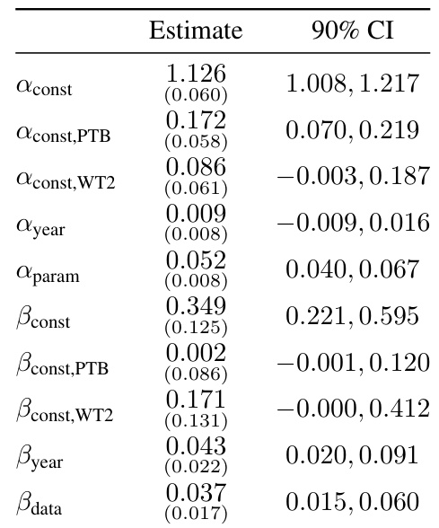
🔼 This table shows the relative contributions of pre-training algorithmic progress and compute scaling to performance gains between pairs of language models. The values are calculated using a Shapley decomposition, which is a technique for fairly assigning the contribution of each factor when their effects are intertwined. Note that parameter efficiency improvements are not shown because they are nearly always zero. The table uses the earliest decoder-only transformer in the dataset as a reference point.
read the caption
Table 1: Attribution of progress to pre-training algorithmic progress and compute scaling between model pairs based on Shapley decomposition in linear space. Numbers may not all add up to 100% due to rounding. These Shapley values are based on point estimates from our preferred model and as such are meant for illustrative purposes only. We omit parameter efficiency improvements from the table since these are almost always 0% and not very informative. The Transformer here is by Baevski and Auli [2018] (the earliest decoder-only transformer we have in our dataset), who modify the original transformer architecture by Vaswani et al. [2017] to be decoder-only.

🔼 This table presents the results of a Shapley value decomposition analysis, which is used to attribute the improvements in language models to either algorithmic progress or compute scaling. The table shows the relative contribution of each factor for several model pairs, considering different starting points and comparing performance gains. Note that due to rounding the values may not always add up to 100%.
read the caption
Table 1: Attribution of progress to pre-training algorithmic progress and compute scaling between model pairs based on Shapley decomposition in linear space. Numbers may not all add up to 100% due to rounding. These Shapley values are based on point estimates from our preferred model and as such are meant for illustrative purposes only. We omit parameter efficiency improvements from the table since these are almost always 0% and not very informative. The Transformer here is by Baevski and Auli [2018] (the earliest decoder-only transformer we have in our dataset), who modify the original transformer architecture by Vaswani et al. [2017] to be decoder-only.
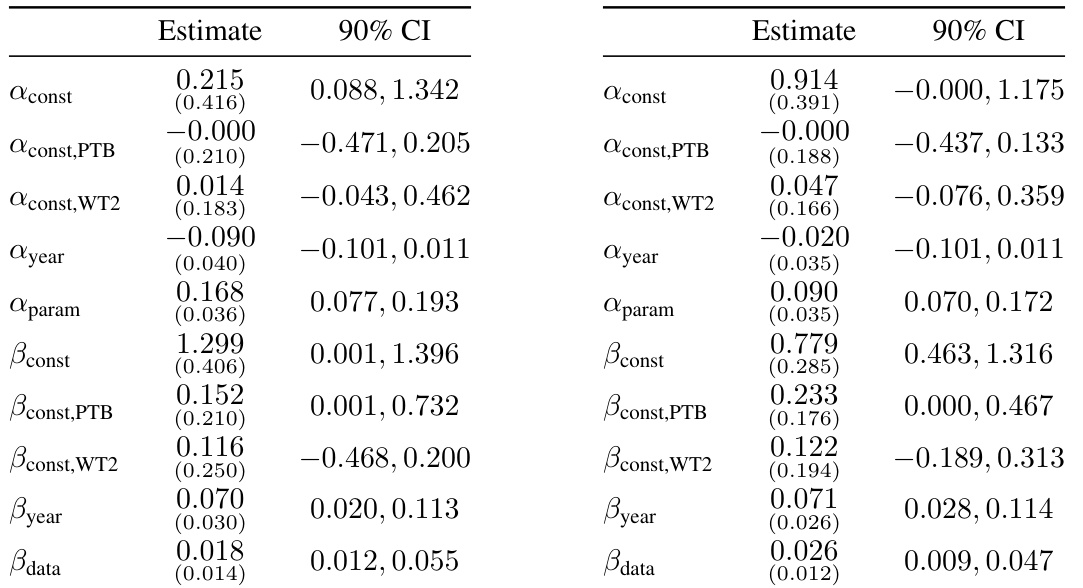
🔼 This table presents a Shapley decomposition of the relative contributions of algorithmic progress and compute scaling to the performance gains observed between pairs of language models. It shows the percentage of performance improvement attributed to each factor for various pairs of models, illustrating the changing balance of these two drivers over time. Note that the Shapley values are based on point estimates and may not always sum to 100% due to rounding.
read the caption
Table 1: Attribution of progress to pre-training algorithmic progress and compute scaling between model pairs based on Shapley decomposition in linear space. Numbers may not all add up to 100% due to rounding. These Shapley values are based on point estimates from our preferred model and as such are meant for illustrative purposes only. We omit parameter efficiency improvements from the table since these are almost always 0% and not very informative. The Transformer here is by Baevski and Auli [2018] (the earliest decoder-only transformer we have in our dataset), who modify the original transformer architecture by Vaswani et al. [2017] to be decoder-only.
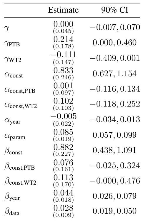
🔼 This table presents a Shapley value decomposition of the contributions of algorithmic progress and compute scaling to the overall progress between different pairs of language models. The Shapley values show the relative contribution of each factor, with parameter efficiency improvements omitted as they are consistently near 0%. The table also notes that the transformer used refers to a specific decoder-only version from 2018 that modifies the original 2017 transformer.
read the caption
Table 1: Attribution of progress to pre-training algorithmic progress and compute scaling between model pairs based on Shapley decomposition in linear space. Numbers may not all add up to 100% due to rounding. These Shapley values are based on point estimates from our preferred model and as such are meant for illustrative purposes only. We omit parameter efficiency improvements from the table since these are almost always 0% and not very informative. The Transformer here is by Baevski and Auli [2018] (the earliest decoder-only transformer we have in our dataset), who modify the original transformer architecture by Vaswani et al. [2017] to be decoder-only.

🔼 This table shows the decomposition of progress in pre-training language models into compute scaling and algorithmic progress for several model pairs. Shapley values are used to attribute the improvements between models to either compute scaling or algorithmic progress. Parameter efficiency improvements are not shown because they are consistently near 0%. The earliest decoder-only transformer model is used as a reference point for the transformer architecture.
read the caption
Table 1: Attribution of progress to pre-training algorithmic progress and compute scaling between model pairs based on Shapley decomposition in linear space. Numbers may not all add up to 100% due to rounding. These Shapley values are based on point estimates from our preferred model and as such are meant for illustrative purposes only. We omit parameter efficiency improvements from the table since these are almost always 0% and not very informative. The Transformer here is by Baevski and Auli [2018] (the earliest decoder-only transformer we have in our dataset), who modify the original transformer architecture by Vaswani et al. [2017] to be decoder-only.
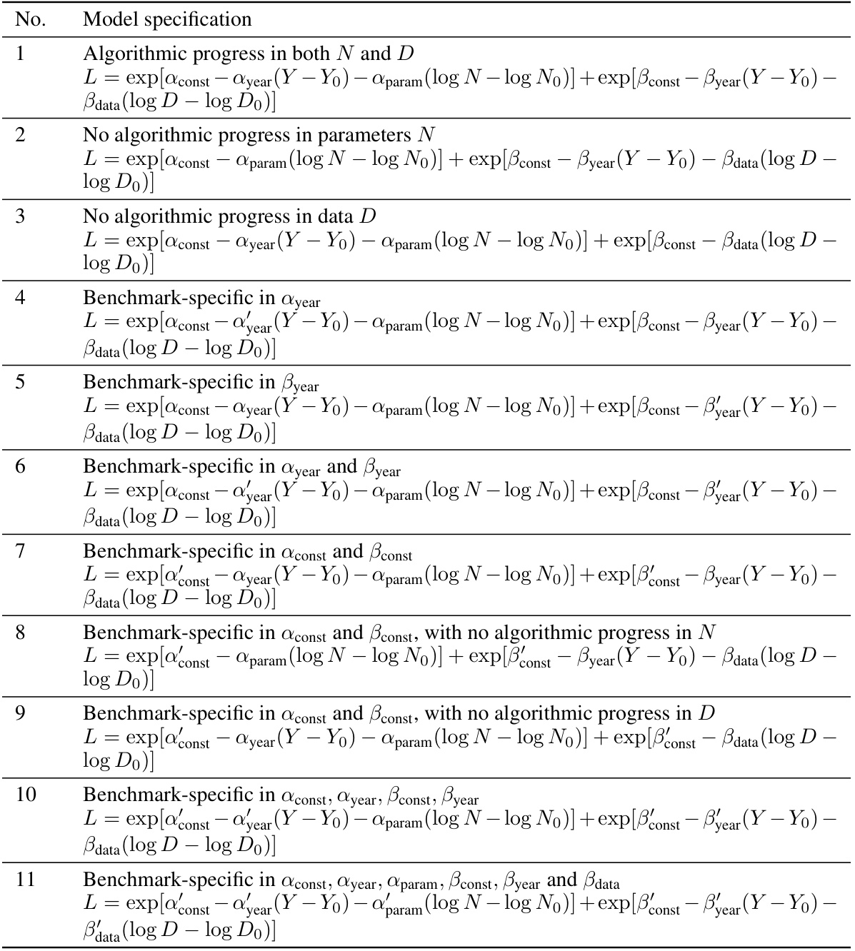
🔼 This table shows the relative contributions of pre-training algorithmic progress and compute scaling to the performance gains between pairs of language models. The Shapley decomposition method is used to attribute the improvements. Note that parameter efficiency gains are omitted due to near-zero values in most cases. The table also specifies the specific transformer model used as a reference point.
read the caption
Table 1: Attribution of progress to pre-training algorithmic progress and compute scaling between model pairs based on Shapley decomposition in linear space. Numbers may not all add up to 100% due to rounding. These Shapley values are based on point estimates from our preferred model and as such are meant for illustrative purposes only. We omit parameter efficiency improvements from the table since these are almost always 0% and not very informative. The Transformer here is by Baevski and Auli [2018] (the earliest decoder-only transformer we have in our dataset), who modify the original transformer architecture by Vaswani et al. [2017] to be decoder-only.
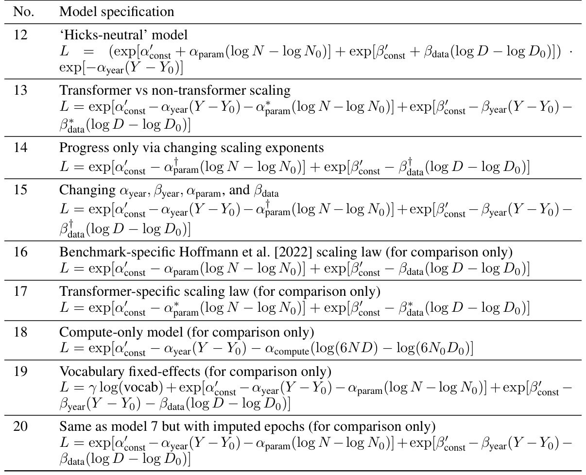
🔼 This table shows the relative contribution of algorithmic progress and compute scaling to the performance improvement between pairs of language models. The Shapley decomposition method is used to fairly allocate the progress between the two factors. Parameter efficiency is omitted because it’s consistently negligible. The table highlights the significant impact of the Transformer architecture.
read the caption
Table 1: Attribution of progress to pre-training algorithmic progress and compute scaling between model pairs based on Shapley decomposition in linear space. Numbers may not all add up to 100% due to rounding. These Shapley values are based on point estimates from our preferred model and as such are meant for illustrative purposes only. We omit parameter efficiency improvements from the table since these are almost always 0% and not very informative. The Transformer here is by Baevski and Auli [2018] (the earliest decoder-only transformer we have in our dataset), who modify the original transformer architecture by Vaswani et al. [2017] to be decoder-only.

🔼 This table shows the relative contributions of algorithmic progress and compute scaling to the performance improvements observed between pairs of language models. The Shapley decomposition method is used to attribute the gains. Note that parameter efficiency improvements are omitted because they are consistently near 0%. The table uses the earliest decoder-only transformer model as a reference point.
read the caption
Table 1: Attribution of progress to pre-training algorithmic progress and compute scaling between model pairs based on Shapley decomposition in linear space. Numbers may not all add up to 100% due to rounding. These Shapley values are based on point estimates from our preferred model and as such are meant for illustrative purposes only. We omit parameter efficiency improvements from the table since these are almost always 0% and not very informative. The Transformer here is by Baevski and Auli [2018] (the earliest decoder-only transformer we have in our dataset), who modify the original transformer architecture by Vaswani et al. [2017] to be decoder-only.
Full paper#
