TL;DR#
Recommender systems often suffer from selection bias, particularly when hidden user features (like age or income) influence both data collection and user feedback, a problem known as hidden confounding. Existing methods for addressing selection bias often fail in these scenarios because they either make strong assumptions about the nature of the hidden confounders or rely on the expensive collection of data from randomized controlled trials. This limits their applicability to real-world situations.
This research paper proposes a new solution called MetaDebias, which utilizes the heterogeneity of observational data to tackle this issue. The core idea is that some data might be collected with complete information (no hidden confounding), while other data may suffer from this bias. MetaDebias uses a meta-learning framework to estimate prediction errors, explicitly model the impact of hidden confounding, and train a model to achieve unbiased predictions using bi-level optimization. Experiments show MetaDebias performs better than existing methods on real-world datasets, highlighting its practical value.
Key Takeaways#
Why does it matter?#
This paper is crucial for researchers in recommendation systems because it tackles the pervasive issue of hidden confounding, a significant challenge in achieving unbiased learning. By introducing MetaDebias, a novel meta-learning approach leveraging heterogeneous observational data, it offers a practical solution to overcome limitations of existing methods. This work opens new avenues for research by exploring heterogeneous data and advancing debiasing techniques.
Visual Insights#

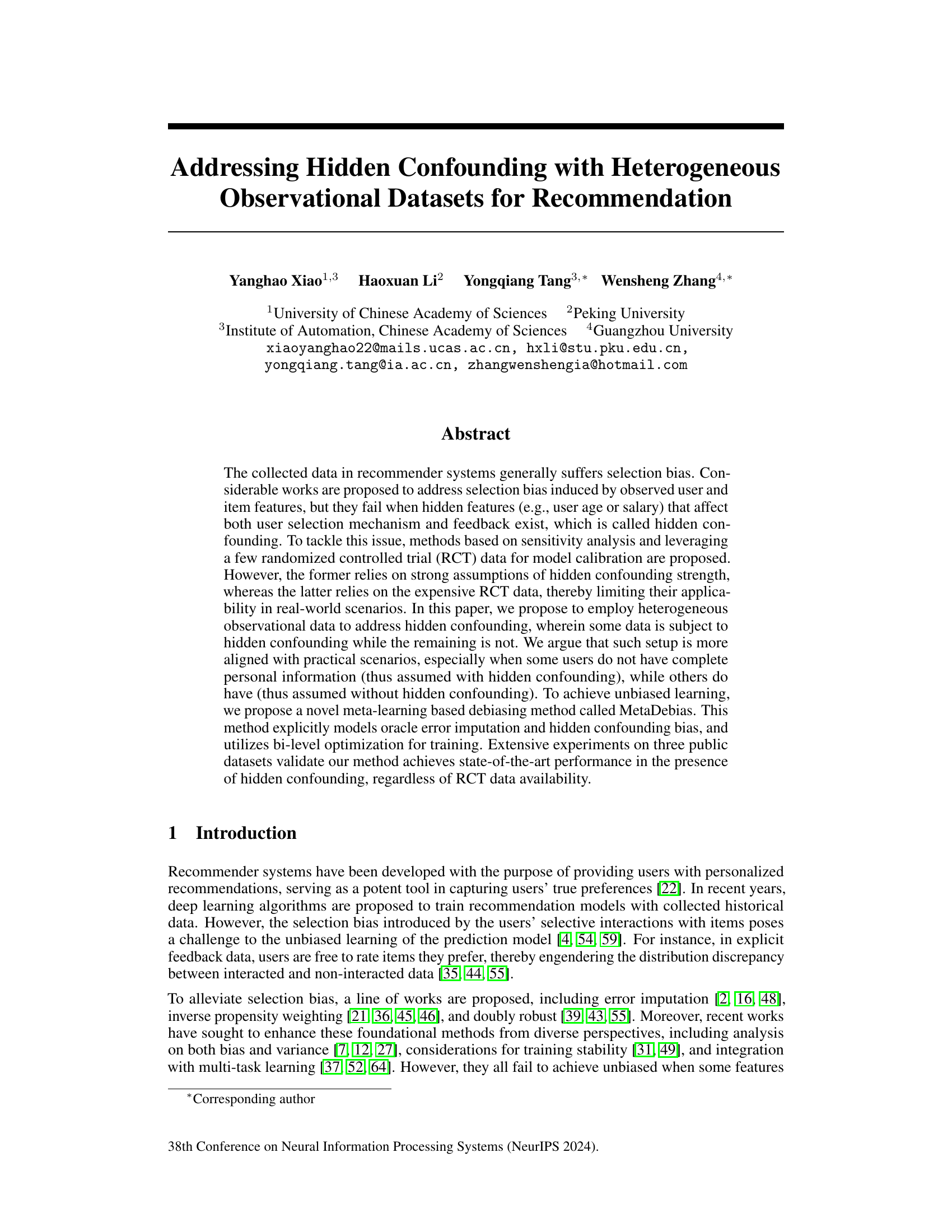
🔼 This figure illustrates two scenarios of user data collection for recommender systems, highlighting the presence or absence of hidden confounding. In the left panel, two example user profiles are presented. Alice provides complete information including optional features (age and salary), while Bob only provides mandatory information (username and gender). This difference is represented by the data source indicator gu,i, where 1 indicates complete data (Alice), and 0 indicates incomplete data (Bob). The right panel displays two causal graphs depicting the relationship between observed and unobserved variables in the presence and absence of hidden confounding. Solid lines indicate observed variables, while dashed lines indicate unobserved variables. The graphs show how the selection bias (MNAR data) is affected by the presence (gu,i=0) or absence (gu,i=1) of hidden confounders (user age or salary), illustrating the challenges of causal inference in this context.
read the caption
Figure 1: Toy examples and causal graphs of heterogeneous observational data, both of which are missing not at random (MNAR) due to the selection bias. In causal graphs, bu,i, Ou,i, ru,i and hu,i denote basic mandatory features, observation, rating and optional features, respectively, where observed and unobserved variables are represented by solid-line and dashed-line circles.
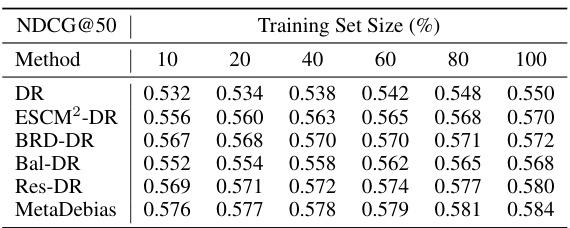
🔼 This table presents the NDCG@K performance on the KUAIREC and YAHOO! R3 datasets using different methods (DR, ESCM2-DR, BRD-DR, Bal-DR, Res-DR, and MetaDebias) with varying training dataset sizes (10%, 20%, 40%, 60%, 80%, and 100%). It demonstrates how the performance of each method changes with the amount of training data.
read the caption
Table 2: Effects of training dataset size on NDCG@K on the KUAIREC and YAHOO! R3 datasets.
In-depth insights#
Hidden Confounding#
Hidden confounding, a significant challenge in recommendation systems, arises when unobserved variables influence both user interaction patterns and feedback mechanisms. Existing debiasing methods often fail under hidden confounding because they rely on observed features alone. Sensitivity analysis addresses this by making strong assumptions about the strength of confounding, while RCT (Randomized Controlled Trial) based approaches require expensive data collection. This paper proposes a novel solution using heterogeneous observational data, which realistically reflects scenarios where some user information is incomplete and assumed to be confounded, while others are complete. By explicitly modeling oracle error imputation and hidden confounding bias in a meta-learning framework, MetaDebias achieves unbiased learning, outperforming existing methods even without RCT data. This approach is of practical importance as it tackles the issue of hidden confounding with readily available data, rather than relying on strong assumptions or expensive data acquisition. The focus on heterogeneous data is crucial, creating a more practical and widely applicable solution for mitigating selection bias in real-world recommendation systems.
MetaDebias Method#
The MetaDebias method is a novel meta-learning approach designed to address the challenge of hidden confounding in recommendation systems. It cleverly leverages heterogeneous observational data, recognizing that real-world datasets often contain a mixture of information completeness. By explicitly modeling both oracle error imputation and hidden confounding bias, and employing a bi-level optimization strategy, MetaDebias aims to achieve unbiased learning. A key strength lies in its ability to work effectively even without the expensive and often unavailable randomized controlled trial (RCT) data, making it a more practical solution for real-world applications. The method’s reliance on identifiable propensity scores and careful estimation of prediction error, differentiated by the presence or absence of hidden confounders, allows it to handle the complexities of incomplete data and biased observations more effectively than existing techniques. The meta-learning framework enhances robustness and accuracy, offering a significant advancement in mitigating bias in recommendation model training.
RCT Data Debate#
The hypothetical “RCT Data Debate” section of a research paper would likely center on the trade-offs between using randomized controlled trials (RCTs) and observational data for causal inference. RCTs offer the gold standard of unbiased causal estimates because they randomly assign participants to treatment and control groups, minimizing confounding. However, RCTs are often expensive, time-consuming, and ethically challenging to conduct, especially in real-world settings like recommendation systems. Observational data, conversely, are readily available but are prone to various biases, including selection bias and confounding. The debate would revolve around how to leverage the strengths of both while mitigating their weaknesses. Methods combining RCT and observational data to calibrate models or estimate causal effects under various assumptions on the nature of confounding would likely be discussed. Furthermore, a core argument would address whether the higher cost and effort of RCTs are justified by the gains in precision, or if sufficiently accurate conclusions can be drawn using advanced statistical techniques on observational data alone. This debate is critical for guiding resource allocation and determining best practices for causal research across various disciplines.
Heterogeneous Data#
The concept of “Heterogeneous Data” in this research paper is crucial for addressing the limitations of existing debiasing methods in recommendation systems. The key idea is that real-world data rarely consists of a single, homogenous dataset. Instead, it often involves multiple data sources with varying levels of completeness and different characteristics (e.g., some users provide complete personal information while others do not). By leveraging this heterogeneity, the authors propose a novel approach to overcome the limitations of existing methods that rely on strong assumptions or require costly randomized controlled trials. This approach directly tackles the hidden confounding problem that often arises when unobserved factors influence both user behavior and item selection. The paper’s innovation lies in its ability to effectively model and utilize data with incomplete information, improving the accuracy and fairness of recommendation models. This framework is a significant step towards developing robust and practical debiasing techniques in real-world applications.
Future Research#
Future research directions stemming from this work on addressing hidden confounding in recommendation systems could explore several promising avenues. Relaxing the reliance on strong assumptions about hidden confounding strength, a limitation of sensitivity analysis methods, is crucial. This could involve developing more robust estimation techniques or exploring alternative identification strategies beyond those presented. Investigating the impact of different feature representation schemes, both for observed and hidden confounders, on the effectiveness of MetaDebias and other debiasing methods would provide valuable insights into the model’s sensitivity to data characteristics. Developing more efficient algorithms to enhance the scalability and reduce computational overhead of MetaDebias for deployment in large-scale, real-world settings is another critical area. Finally, extending the framework to incorporate temporal dynamics, addressing the evolving nature of user preferences and item popularity over time, would improve the practical applicability and long-term value of the proposed method.
More visual insights#
More on figures
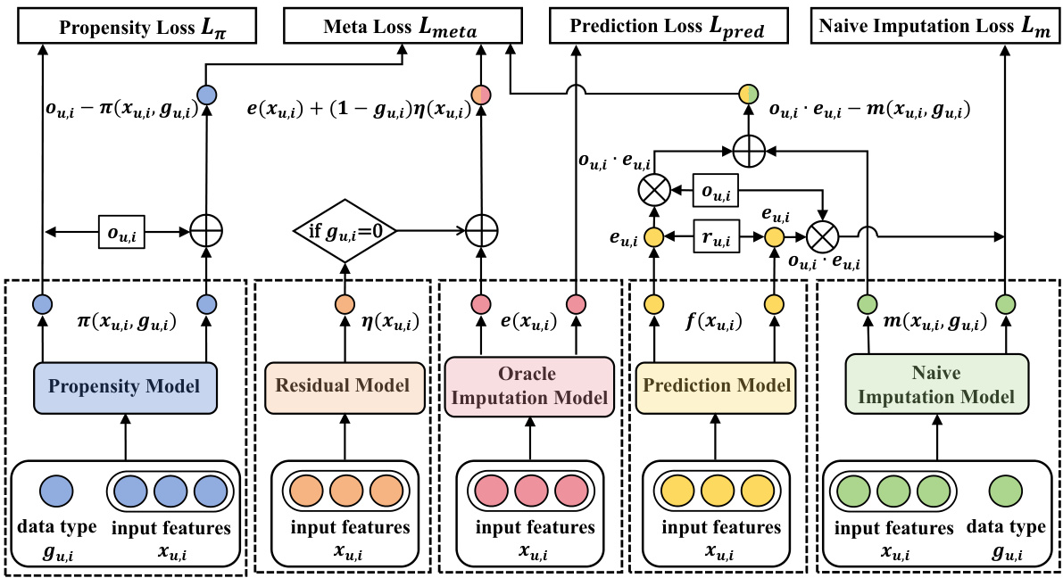
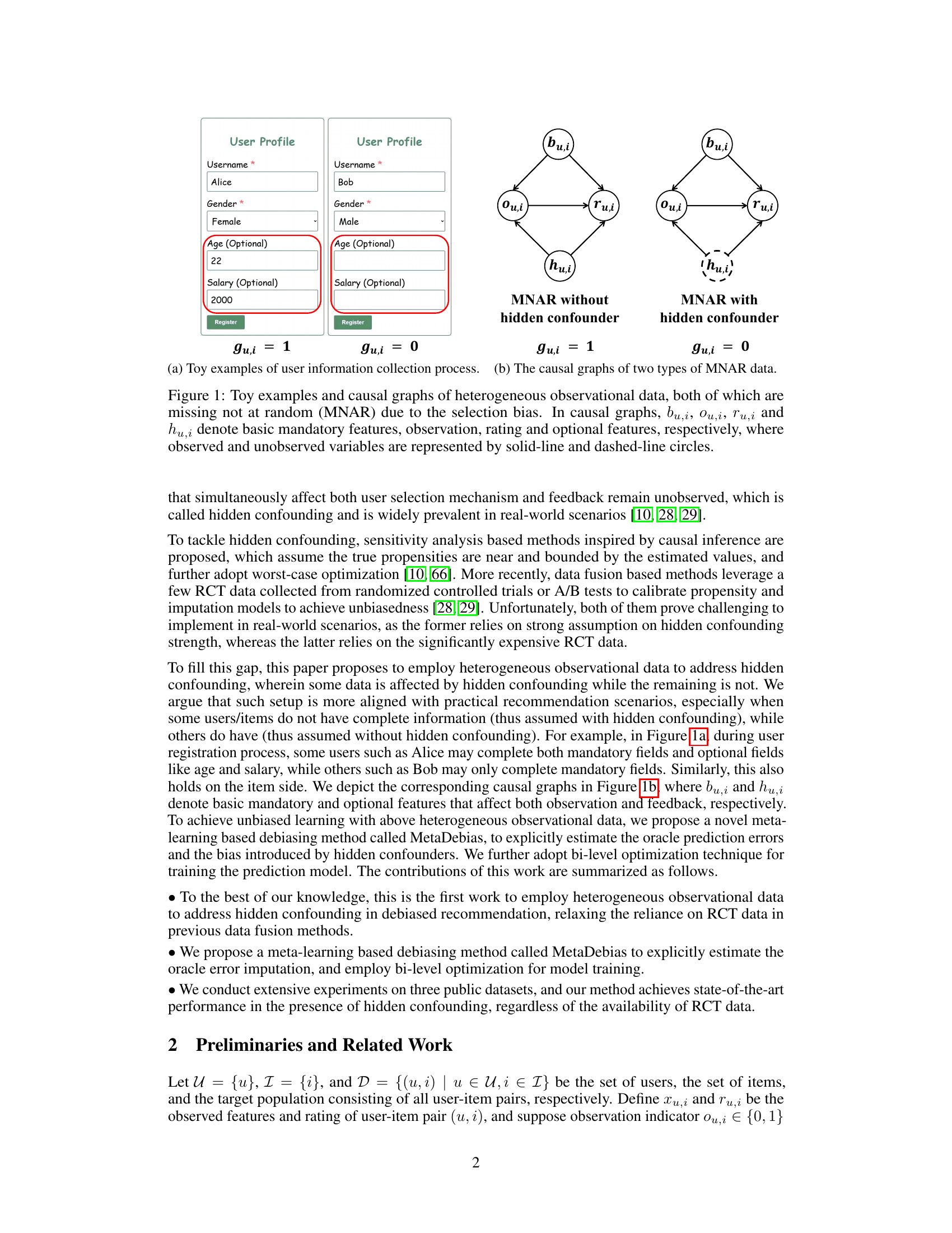
🔼 The figure shows the architecture of the MetaDebias model, which addresses selection bias in recommendation systems in the presence of hidden confounders. The model consists of five sub-models: a propensity model, a residual model, an oracle imputation model, a prediction model, and a naive imputation model. The propensity model estimates the probability of observing a rating given the input features and the data source indicator (gu,i). The residual model captures the difference in prediction errors between subgroups with and without hidden confounders. The oracle imputation model estimates the oracle prediction error on all user-item pairs. The prediction model predicts the true ratings and the naive imputation model estimates the naive prediction error based on the observed features. The different sub-models are connected through a series of operations which allow the model to learn from heterogeneous data with both observed and hidden confounders and make unbiased predictions.
read the caption
Figure 2: Architecture of MetaDebias to address selection bias in the presence of hidden confounding.
🔼 This figure shows the architecture of the MetaDebias model, illustrating how it addresses selection bias in the presence of hidden confounding. The model consists of several components: a propensity model (predicting the probability of observing a rating), a residual model (modeling the difference in prediction error between observed and unobserved data), an oracle imputation model (estimating the true prediction error), a prediction model (predicting ratings), and a naive imputation model (a simpler imputation model used in the training process). The model utilizes a meta-learning approach, optimizing the oracle imputation model to improve the performance of the prediction model. The input includes features (Xu,i), a data source indicator (gu,i), and the observed rating (Ou,i * ru,i).
read the caption
Figure 2: Architecture of MetaDebias to address selection bias in the presence of hidden confounding.

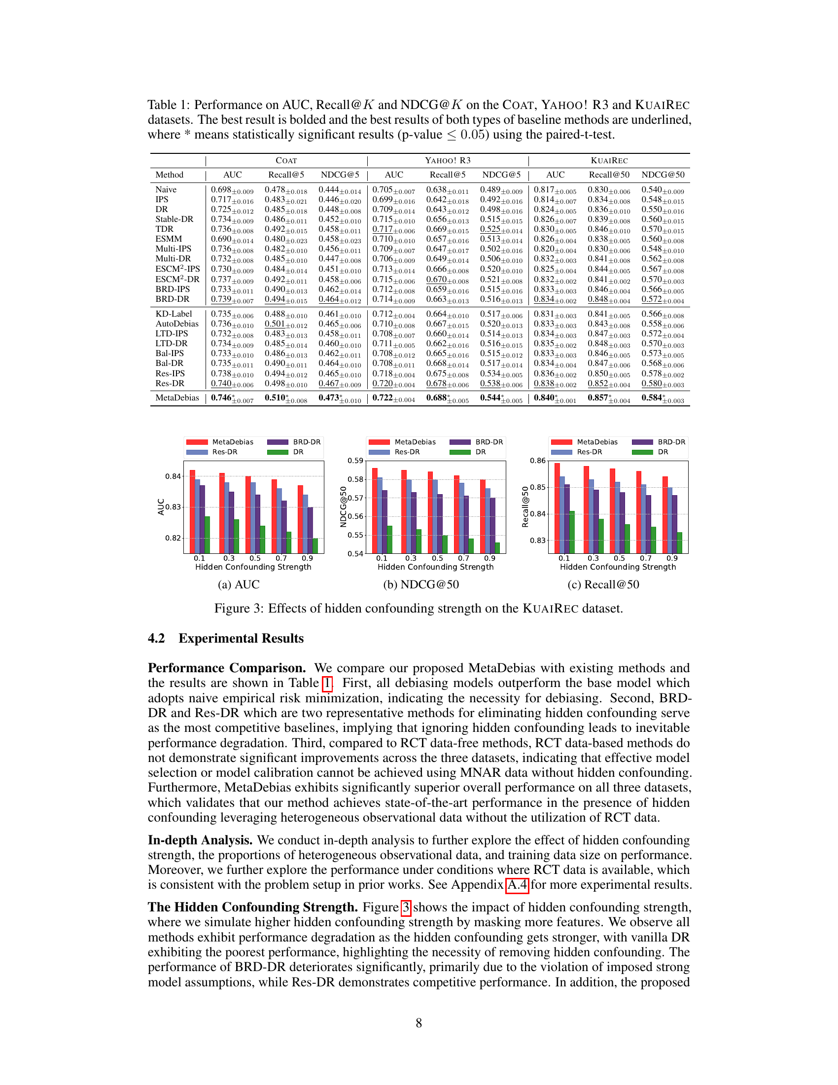
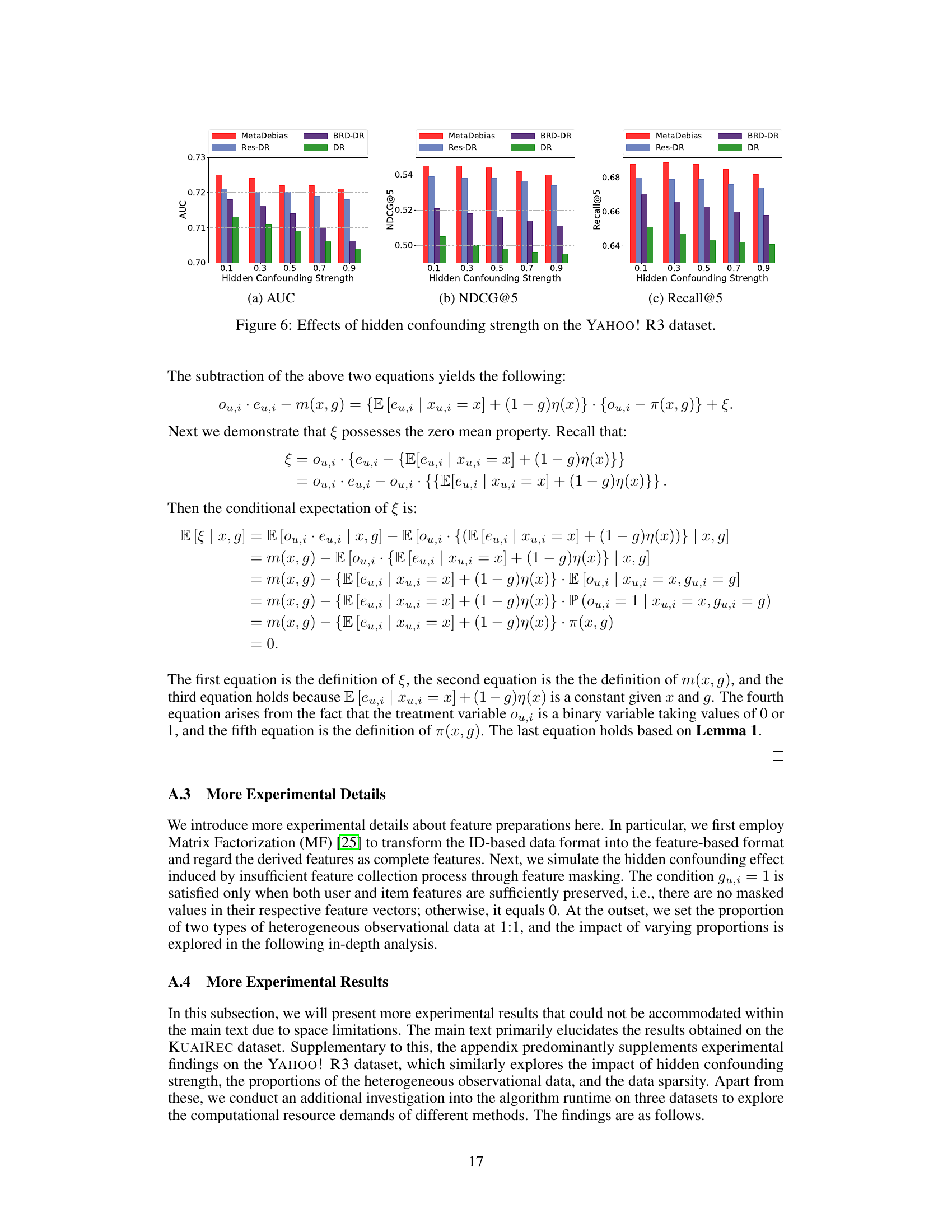
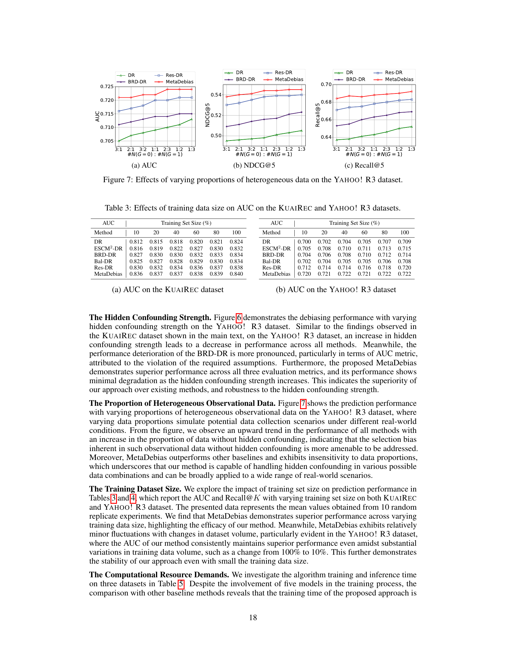
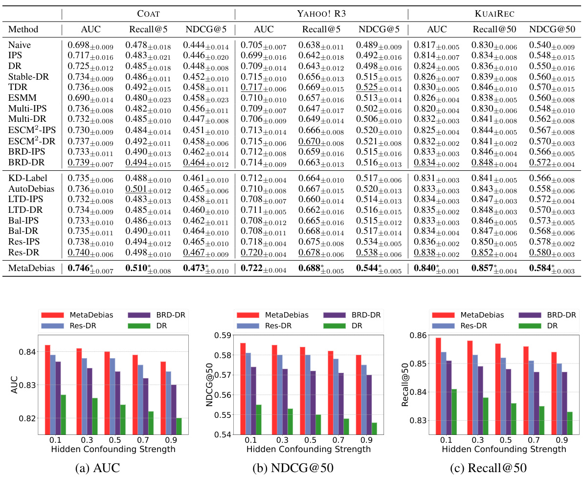
🔼 This figure shows the impact of hidden confounding strength on the KUAIREC dataset. The x-axis represents the hidden confounding strength, ranging from 0.1 to 0.9. The y-axis shows the performance metrics: AUC, NDCG@50, and Recall@50. The different colored lines represent different debiased recommendation methods (DR, BRD-DR, Res-DR, and MetaDebias). The figure demonstrates how the performance of all methods degrades as the hidden confounding strength increases. MetaDebias shows comparatively better performance compared to other methods.
read the caption
Figure 3: Effects of hidden confounding strength on the KUAIREC dataset.

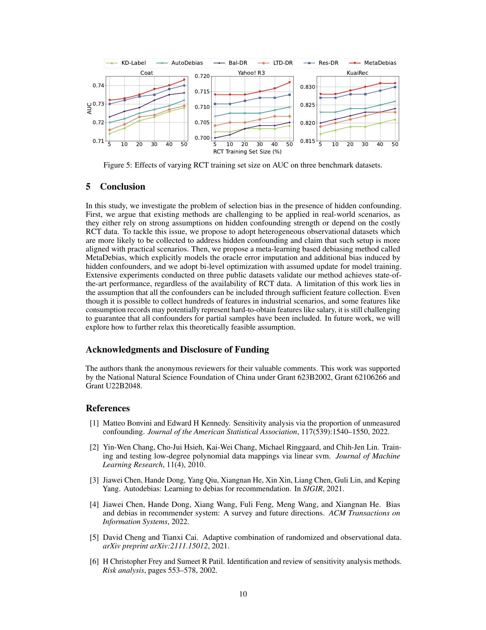
🔼 This figure shows the impact of varying the percentage of RCT training data on the AUC (Area Under the Curve) performance metric across three benchmark datasets: Coat, Yahoo! R3, and KuaiRec. Each line represents a different debiasing method (KD-Label, AutoDebias, Bal-DR, LTD-DR, Res-DR, and MetaDebias). The x-axis shows the percentage of RCT data used, and the y-axis displays the AUC scores. The figure demonstrates how the performance of each method changes as the amount of RCT data increases, highlighting the relative effectiveness of each debiasing technique in the presence of RCT data.
read the caption
Figure 5: Effects of varying RCT training set size on AUC on three benchmark datasets.

🔼 This figure shows the impact of hidden confounding strength on the KUAIREC dataset. The x-axis represents the strength of hidden confounding, and the y-axis shows the performance metrics (AUC, NDCG@50, Recall@50). The results show that as the hidden confounding strength increases, the performance of all methods degrades. However, MetaDebias shows superior performance in handling the confounding compared to other methods.
read the caption
Figure 3: Effects of hidden confounding strength on the KUAIREC dataset.

🔼 This figure shows the impact of hidden confounding strength on the KUAIREC dataset. The x-axis represents the strength of hidden confounding, and the y-axis shows the performance metrics (AUC, NDCG@50, and Recall@50). The different colored bars represent different debiasing methods (DR, BRD-DR, Res-DR, and MetaDebias). The results show how performance degrades as hidden confounding increases, illustrating the effectiveness of the MetaDebias approach, which maintains a higher performance even with stronger confounding.
read the caption
Figure 3: Effects of hidden confounding strength on the KUAIREC dataset.
More on tables

🔼 This table shows the NDCG@K scores achieved by different recommendation models on the KUAIREC and YAHOO! R3 datasets with varying training dataset sizes (10%, 20%, 40%, 60%, 80%, and 100%). It demonstrates the effect of the training data size on the performance of each model in terms of NDCG@K. The results highlight the impact of data availability on the model’s ability to effectively learn and predict user preferences.
read the caption
Table 2: Effects of training dataset size on NDCG@K on the KUAIREC and YAHOO! R3 datasets.

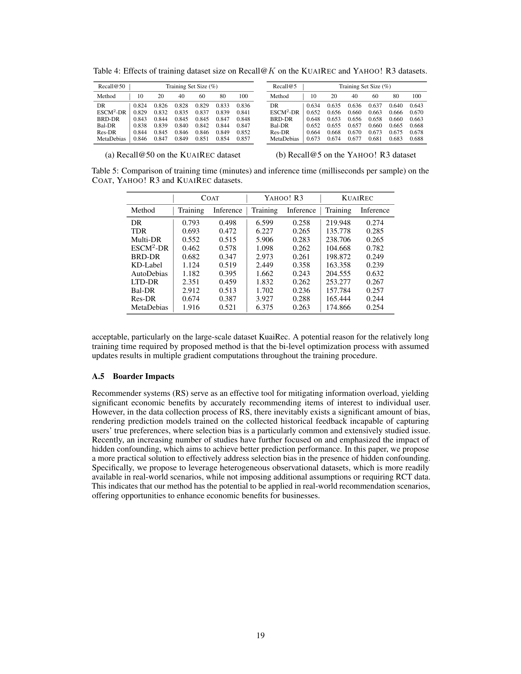
🔼 This table presents the results of an experiment evaluating the impact of training dataset size on the Area Under the Curve (AUC) metric. The experiment was conducted on two datasets, KUAIREC and YAHOO! R3. Multiple methods (DR, ESCM²-DR, BRD-DR, Bal-DR, Res-DR, and MetaDebias) were compared, showing their AUC scores at various training dataset sizes (10%, 20%, 40%, 60%, 80%, and 100%). The table allows for a comparison of the performance of different debiasing methods under varying data availability.
read the caption
Table 3: Effects of training data size on AUC on the KUAIREC and YAHOO! R3 datasets.

🔼 This table presents the results of an experiment evaluating the impact of training dataset size on the Area Under the Curve (AUC) metric. The experiment was conducted on two datasets: KUAIREC and YAHOO! R3. Multiple methods (DR, ESCM²-DR, BRD-DR, Bal-DR, Res-DR, and MetaDebias) were compared using training datasets of varying sizes (10%, 20%, 40%, 60%, 80%, and 100%). The AUC values for each method and dataset size are shown, illustrating the effect of data quantity on model performance.
read the caption
Table 3: Effects of training data size on AUC on the KUAIREC and YAHOO! R3 datasets.

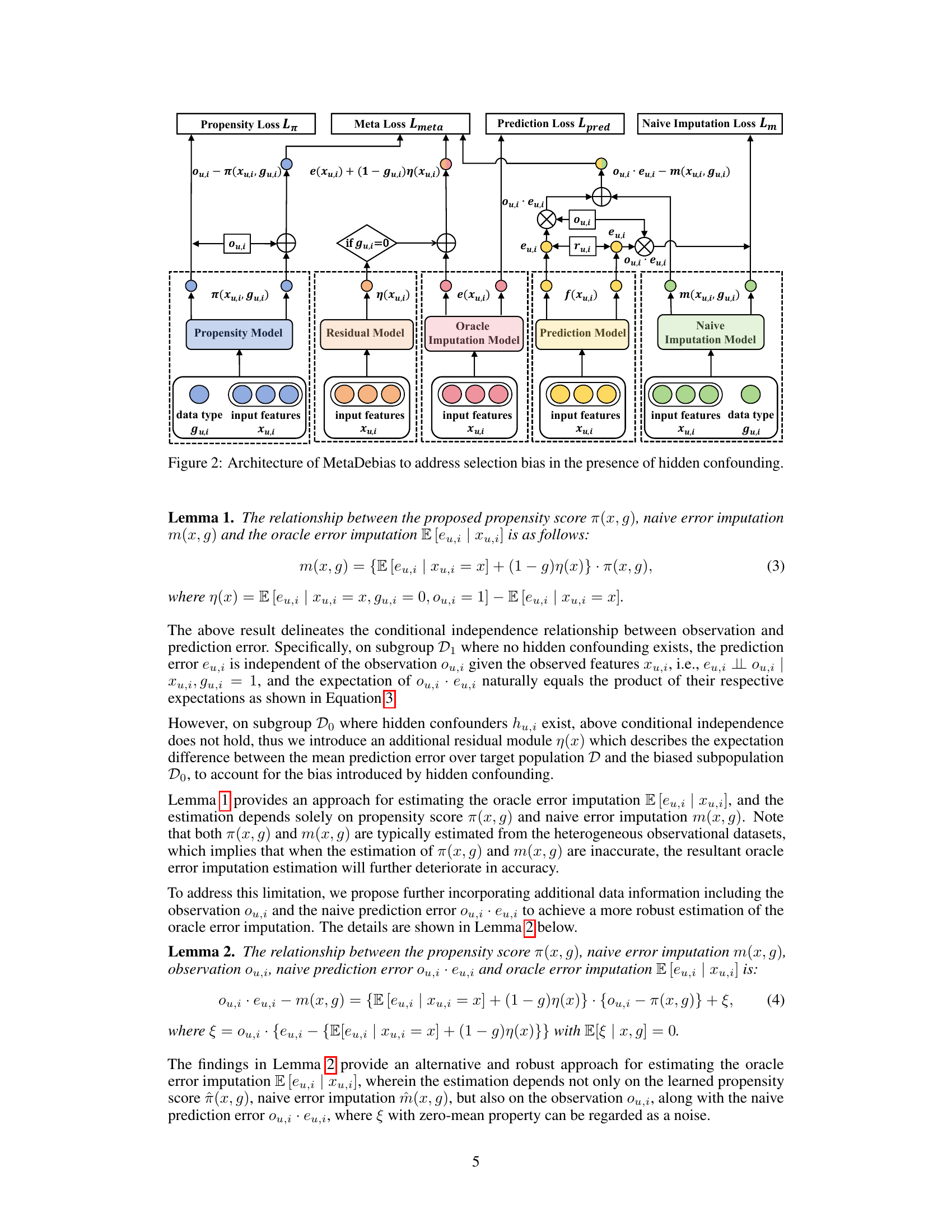
🔼 This table presents the performance comparison of different recommendation models on three benchmark datasets (COAT, YAHOO! R3, and KUAIREC) across three evaluation metrics: AUC, Recall@K, and NDCG@K. The best-performing model for each metric and dataset is highlighted in bold. Additionally, the best performing model among the RCT data-free and RCT data-based methods are underlined. The ‘*’ indicates statistically significant differences (p<0.05) based on paired t-tests.
read the caption
Table 1: Performance on AUC, Recall@K and NDCG@K on the COAT, YAHOO! R3 and KUAIREC datasets. The best result is bolded and the best results of both types of baseline methods are underlined, where * means statistically significant results (p-value < 0.05) using the paired-t-test.
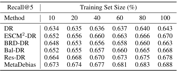
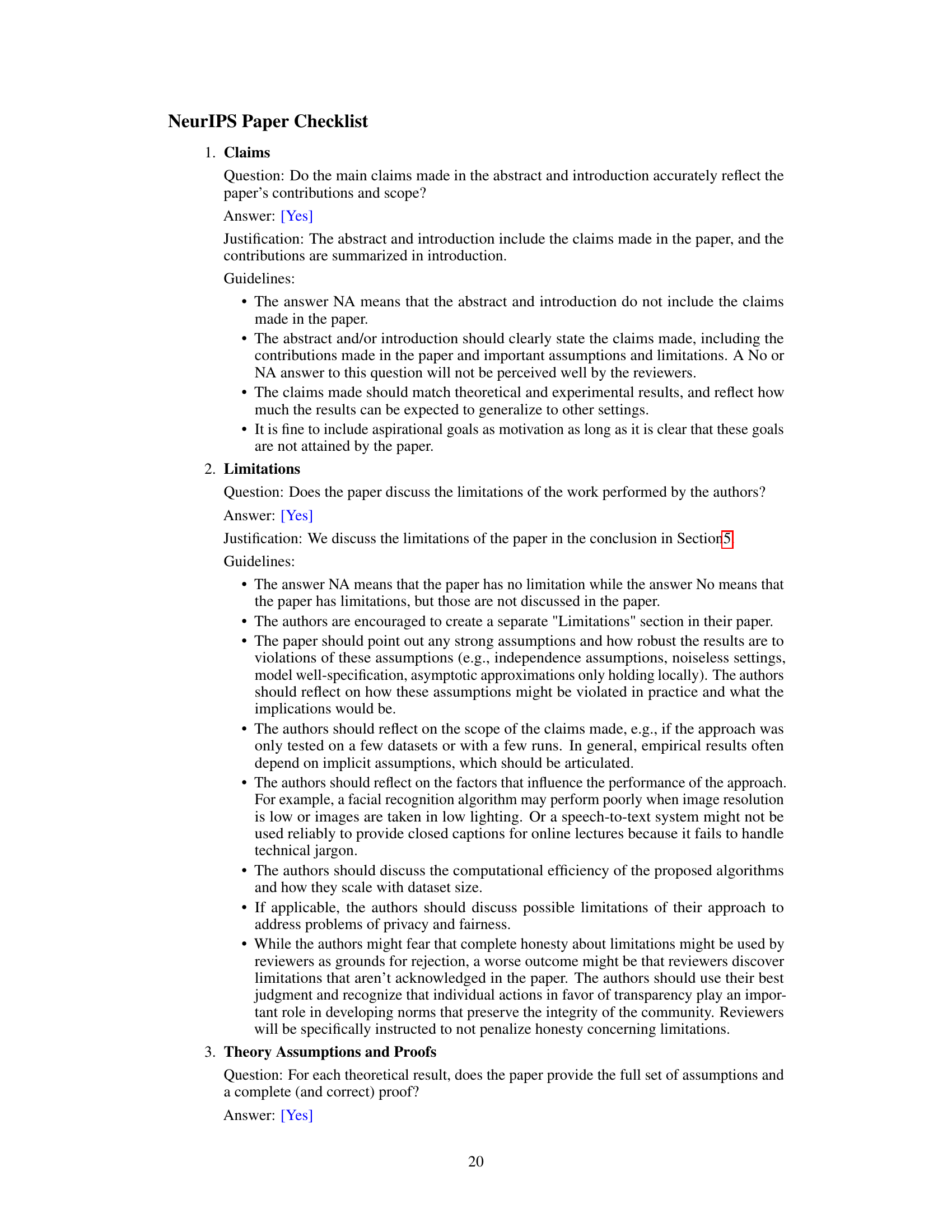
🔼 This table shows the performance (Recall@K) of different recommendation models under varying training dataset sizes. The models are evaluated on two datasets: KUAIREC and YAHOO! R3. The results demonstrate how the model’s performance changes as the amount of training data increases, indicating the impact of data size on model training and generalization. The table allows for a comparison of different model’s sensitivity to varying training data amounts. The Recall@K metric provides insights into each models’ ability to accurately retrieve relevant items in the top K recommendations.
read the caption
Table 4: Effects of training dataset size on Recall@K on the KUAIREC and YAHOO! R3 datasets.
🔼 This table presents the performance comparison of different recommendation models on three datasets (COAT, YAHOO! R3, and KUAIREC) using three evaluation metrics (AUC, Recall@K, NDCG@K). The best overall performance for each metric and dataset is shown in bold, while the best results among both RCT data-free and RCT data-based methods are underlined. Statistical significance (p<0.05) using paired t-test is indicated with an asterisk.
read the caption
Table 1: Performance on AUC, Recall@K and NDCG@K on the COAT, YAHOO! R3 and KUAIREC datasets. The best result is bolded and the best results of both types of baseline methods are underlined, where * means statistically significant results (p-value < 0.05) using the paired-t-test.
Full paper#
