TL;DR#
Many scientific studies involve discrete data with unobserved (latent) variables. Understanding causal relationships among these latent variables is crucial, but existing methods often struggle with non-linear relationships or complex structures. This limits their applicability in many real-world scenarios. Current approaches often rely on strong assumptions like linearity, which may not hold in practice.
This paper tackles this limitation by proposing a novel method using a tensor rank condition. The authors demonstrate that the rank of a contingency table is determined by the minimum support of a specific conditional set that separates the observed variables. This allows for the identification of latent variables and their causal structure. The proposed algorithm is tested on simulated and real-world data, showing its efficiency and robustness in uncovering complex causal structures within discrete latent variable models.
Key Takeaways#
Why does it matter?#
This paper is crucial for researchers working with discrete data and latent variables, which are common in various fields like social sciences and psychology. The proposed tensor rank condition and accompanying algorithm provide a novel and efficient method for learning complex causal structures, solving a long-standing challenge in causal discovery. This opens up new avenues for research, especially in handling non-linear and high-dimensional data, and offers practical tools for various applications.
Visual Insights#
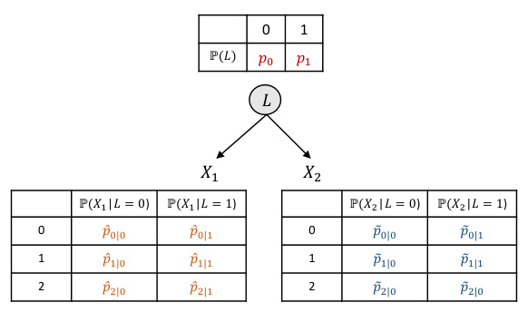
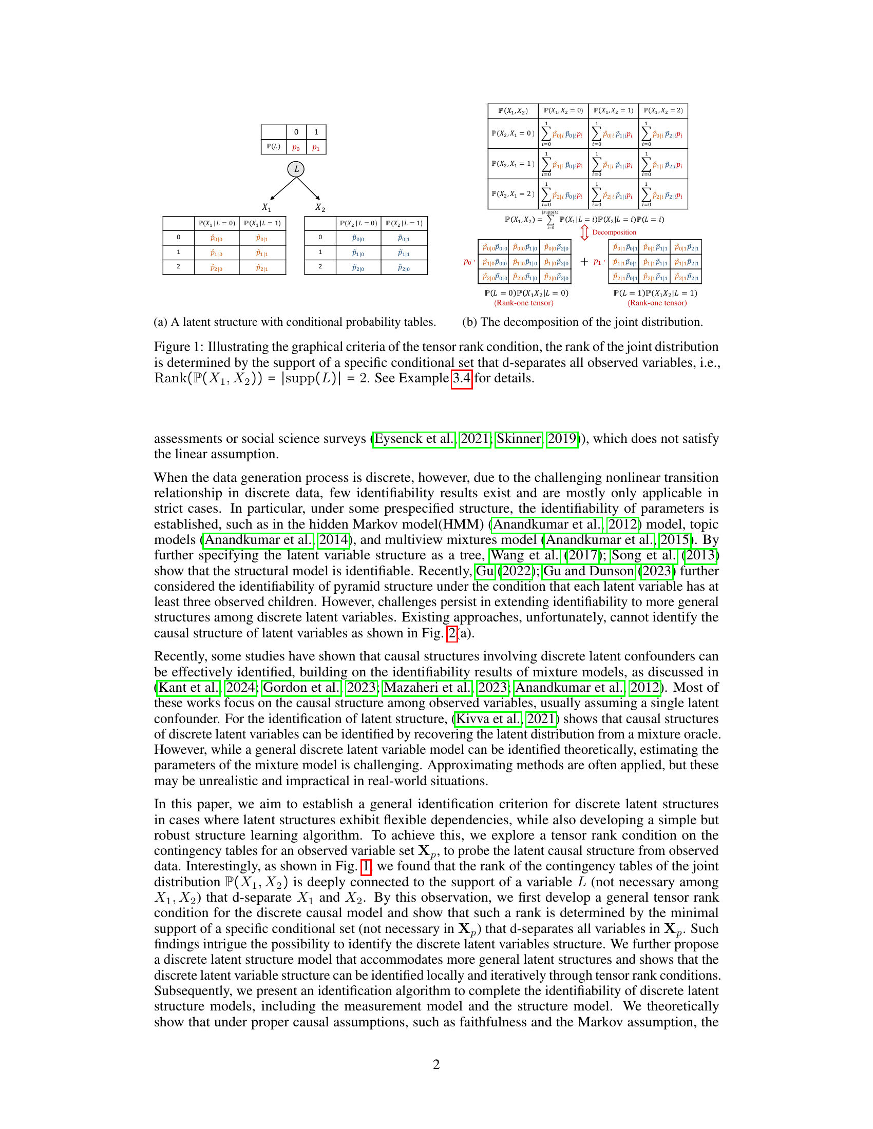
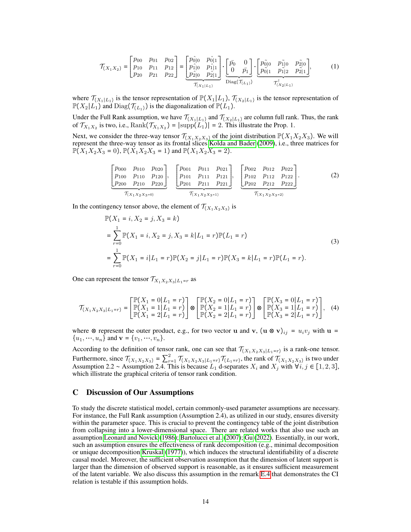
🔼 This figure illustrates the relationship between the tensor rank of the joint distribution of observed variables (X1, X2) and the support of a latent variable (L) that d-separates them. It shows how the rank of the joint distribution is equivalent to the size of the support (number of possible values) of the latent variable that renders the observed variables conditionally independent. The example uses a simple latent variable structure with conditional probability tables to demonstrate the concept. The figure demonstrates the tensor decomposition into rank-one tensors, highlighting that the number of these rank-one tensors is equal to the cardinality of the latent variable’s support. This is a key element of the tensor rank condition described in the paper.
read the caption
Figure 1: Illustrating the graphical criteria of the tensor rank condition, the rank of the joint distribution is determined by the support of a specific conditional set that d-separates all observed variables, i.e., Rank(P(X1, X2)) = |supp(L)| = 2. See Example 3.4 for details.

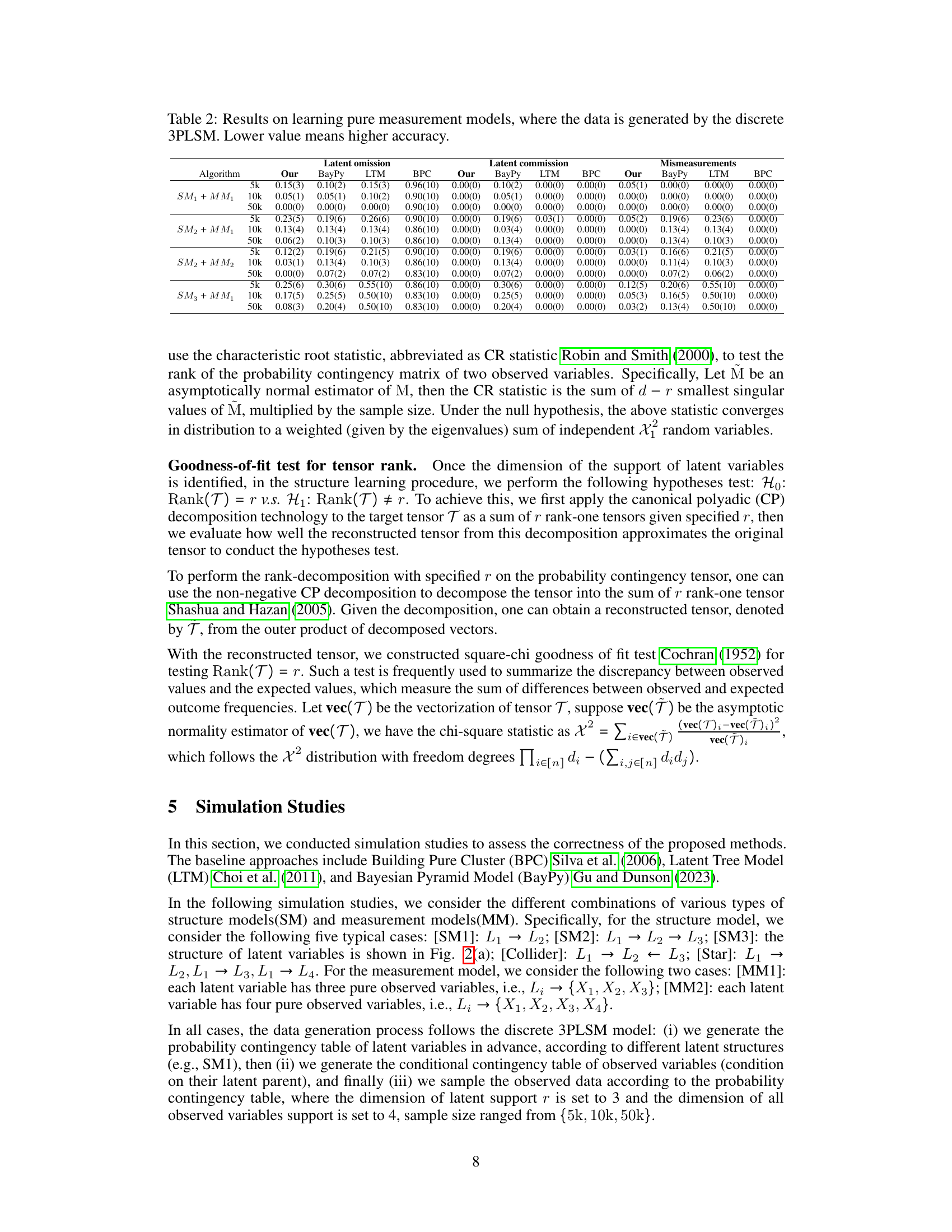
🔼 This table presents the results of experiments evaluating the performance of different algorithms in learning pure measurement models. The data was generated using the discrete 3PLSM model. The algorithms were compared based on three metrics: latent omission, latent commission, and mismeasurement. Lower values indicate better performance. The table includes results for different sample sizes (5k, 10k, 50k) and different model configurations (SM1+MM1, SM2+MM1, SM3+MM1, SM2+MM2, SM3+MM2).
read the caption
Table 2: Results on learning pure measurement models, where the data is generated by the discrete 3PLSM. Lower value means higher accuracy.
In-depth insights#
Tensor Rank & Causality#
The concept of ‘Tensor Rank & Causality’ merges tensor decomposition techniques with causal inference. Tensor rank, a measure of the complexity of a tensor, is proposed as a key indicator of causal relationships. The intuition is that the minimal rank decomposition of a joint probability distribution reveals underlying causal structures, linking tensor rank to the minimal support size of a conditional set that d-separates observed variables. This approach allows for identifying latent variables and their causal relationships, handling non-linearity and complex latent structures that often challenge traditional methods. The faithfulness assumption is crucial, ensuring that all statistical independence relations reflect true causal dependencies. The algorithm leverages tensor rank conditions iteratively, identifying causal clusters and then inferring the causal structure among latent variables. This framework represents a significant step toward causal discovery in discrete data, expanding its application scope beyond linear latent variable models. However, scalability to high-dimensional data and the computational cost of tensor decomposition remain challenges. Future work can focus on addressing these limitations and exploring the use of approximation methods to enhance efficiency.
Discrete Latent Models#
Discrete latent variable models address the challenge of uncovering causal relationships among unobservable variables in data exhibiting discrete characteristics. These models are crucial when dealing with categorical data, where traditional linear methods are often inadequate. Key challenges include ensuring model identifiability (guaranteeing a unique solution) and developing efficient algorithms for structure learning. Tensor rank conditions have been explored as a powerful tool in identifying latent structures, leveraging the mathematical properties of tensors to infer the underlying causal network. The choice of assumptions (e.g., faithfulness, Markov conditions) significantly impacts identifiability and adds complexity. Discrete 3PLSM (three-pure-children latent structure model) provides a framework with specific structural constraints to achieve identifiability, but this model’s limited generality remains a consideration. Future research could focus on relaxing constraints, and developing more robust, scalable algorithms to address high-dimensional datasets and complex latent structures.
Tensor Rank Testing#
Tensor rank testing, in the context of this research paper focusing on learning discrete latent variable structures, is a crucial step for identifying the underlying causal relationships. The core idea revolves around the connection between the rank of a tensor representation of observed variable data and the minimal support size of a conditional variable set. This connection is theoretically grounded and allows for identifying latent variables, essentially acting as a graphical criteria for discovering causal structures. The rank is determined by finding the minimal set that d-separates all variables in the observed set. Practical tensor rank testing involves challenges, such as estimating the rank of the contingency tables reliably, and there may be computational limitations in real-world scenarios with high-dimensional data. The effectiveness of this technique heavily depends on assumptions like faithfulness and the Markov condition, highlighting the need for careful consideration of these assumptions when interpreting the results. The use of goodness-of-fit tests for validating the estimated rank further underscores the importance of addressing potential inaccuracies in the rank estimation procedure.
Structure Learning Algo#
A structure learning algorithm, in the context of learning discrete latent variable structures, is crucial for uncovering the underlying causal relationships between latent variables. The algorithm’s effectiveness hinges on its ability to handle the complexities of discrete data and non-linear relationships, unlike linear approaches which often fail in these scenarios. A key aspect of such an algorithm would be its identification process. This often involves leveraging tensor rank conditions on contingency tables of observed variables to pinpoint latent variables. By analyzing the rank, the algorithm aims to discover the minimal set of variables that d-separates all observed variables, thus revealing latent structure. The algorithm must incorporate efficient methods for calculating tensor rank and effectively testing conditional independence to ensure accuracy and robustness. Ultimately, a robust structure learning algorithm will significantly advance causal discovery research, especially when dealing with discrete and complex latent variable systems.
High-dim. Challenges#
High-dimensional data presents significant challenges in causal discovery, particularly when dealing with latent variables. The curse of dimensionality implies that the number of possible causal structures grows exponentially with the number of variables, making exhaustive search computationally infeasible. High-dimensional data often suffers from sparsity, meaning many variable pairs are only weakly associated or not associated at all, thus hindering the identification of genuine causal relationships. Existing methods often rely on strong assumptions, such as linearity or Gaussianity, which frequently do not hold for real-world datasets. The presence of latent variables adds further complexity, as unobserved confounders can induce spurious associations between observed variables, potentially leading to incorrect causal inferences. Therefore, addressing high-dimensionality requires innovative algorithmic approaches, potentially leveraging sparsity assumptions or advanced methods such as tensor decomposition, which can better handle the complexities of high-dimensional discrete data and latent variable models. Robustness to noise and model misspecification is also critical, as high-dimensional data is often noisy and may not perfectly adhere to the assumed model. Novel techniques incorporating regularization or incorporating domain knowledge can be considered to improve reliability and accuracy.
More visual insights#
More on figures
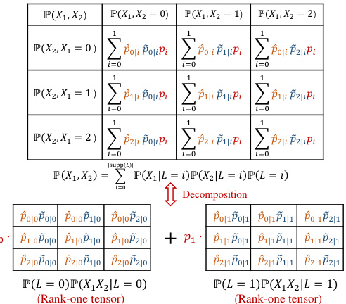
🔼 This figure illustrates how the tensor rank condition relates to the graphical structure of a discrete causal model. Panel (a) shows a simple model with a latent variable L influencing two observed variables, X1 and X2. Panel (b) demonstrates the decomposition of the joint distribution P(X1, X2) into a sum of rank-one tensors. The rank of this tensor (which is 2 in this example) is equal to the size of the support of the latent variable L, demonstrating that the minimum support of a variable that d-separates the observed variables determines the tensor rank.
read the caption
Figure 1: Illustrating the graphical criteria of the tensor rank condition, the rank of the joint distribution is determined by the support of a specific conditional set that d-separates all observed variables, i.e., Rank(P(X1, X2)) = |supp(L)| = 2. See Example 3.4 for details.

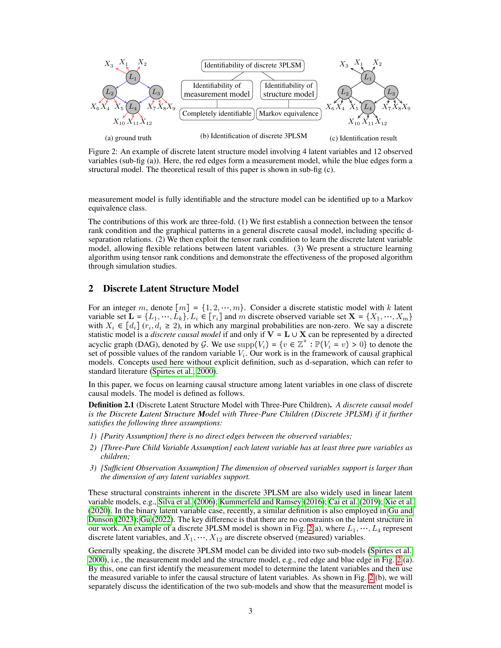
🔼 This figure shows an example of a discrete latent structure model with 4 latent variables and 12 observed variables. Subfigure (a) displays the ground truth model, with red edges representing the measurement model (relationships between latent and observed variables) and blue edges representing the structural model (relationships between latent variables). Subfigure (b) illustrates the identifiability results for the discrete 3PLSM (Discrete Latent Structure Model with Three-Pure Children), showing how the measurement model is completely identifiable and the structure model is identifiable up to Markov equivalence. Subfigure (c) shows the final identification result.
read the caption
Figure 2: An example of discrete latent structure model involving 4 latent variables and 12 observed variables (sub-fig (a)). Here, the red edges form a measurement model, while the blue edges form a structural model. The theoretical result of this paper is shown in sub-fig (c).

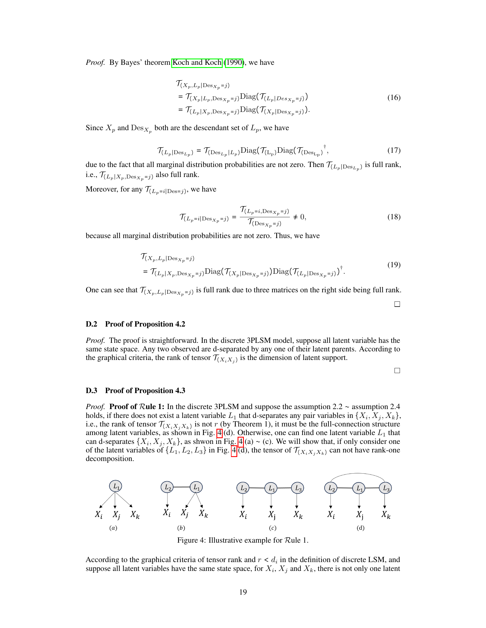
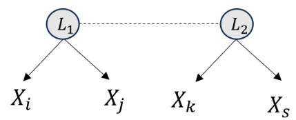
🔼 This figure illustrates four different scenarios of relationships between three observed variables (Xi, Xj, Xk) and their latent variables. (a), (b), and (c) represent cases where Xi, Xj, and Xk share a common latent parent and thus form a causal cluster. In contrast, (d) shows a case where Xi, Xj, Xk do not share a common latent parent. This example helps to explain the criteria of causal cluster identification, as proposed in Rule 1 of the paper.
read the caption
Figure 4: Illustrative example for Rule 1.
🔼 This figure illustrates a simple discrete causal model with a latent variable L influencing two observed variables, X1 and X2. The joint distribution P(X1,X2) can be decomposed into a sum of rank-one tensors, where the number of rank-one tensors equals the support size of the latent variable L. The tensor rank condition states that the minimum support size of a conditional variable set that d-separates all observed variables is the rank of their joint probability distribution. This figure visually demonstrates this condition, showing the connection between the tensor rank and the d-separation relations in a causal graph.
read the caption
Figure 1: Illustrating the graphical criteria of the tensor rank condition, the rank of the joint distribution is determined by the support of a specific conditional set that d-separates all observed variables, i.e., Rank(P(X1, X2)) = |supp(L)| = 2. See Example 3.4 for details.
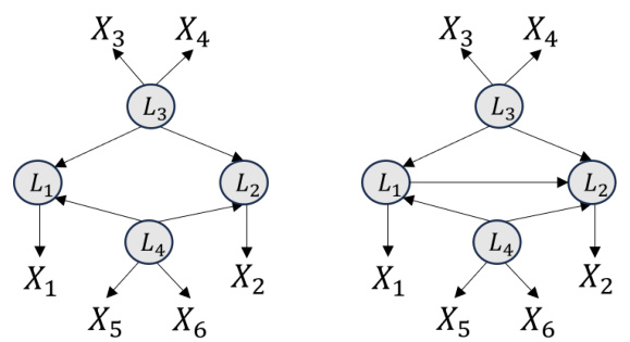
🔼 This figure presents two graphical models. Sub-figure (a) shows a ground truth model with four latent variables (L1, L2, L3, L4) and twelve observed variables (X1-X12). The red edges represent the measurement model, indicating how the latent variables influence the observed ones. The blue edges illustrate the structural model, showing the relationships between the latent variables. Sub-figure (c) presents the identification results showing that both the measurement model and the structural model are identifiable.
read the caption
Figure 2: An example of discrete latent structure model involving 4 latent variables and 12 observed variables (sub-fig (a)). Here, the red edges form a measurement model, while the blue edges form a structural model.
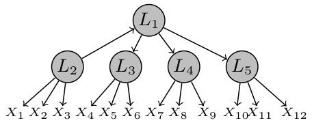
🔼 This figure illustrates an example of a discrete latent structure model (3PLSM) with four latent variables and twelve observed variables. Subfigure (a) shows the ground truth of the model, with red edges representing the measurement model (links between latent and observed variables) and blue edges representing the structural model (links between latent variables). Subfigure (b) illustrates the identification process for the discrete 3PLSM. Subfigure (c) presents the theoretical identification result, showing what can be identified using the methods proposed in the paper.
read the caption
Figure 2: An example of discrete latent structure model involving 4 latent variables and 12 observed variables (sub-fig (a)). Here, the red edges form a measurement model, while the blue edges form a structural model. The theoretical result of this paper is shown in sub-fig (c).
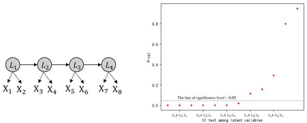
🔼 The figure shows the results of conditional independence (CI) tests among latent variables using a goodness-of-fit test. A chain structure with four latent variables (L1, L2, L3, L4), each with two observed children, is used. The plot shows p-values for various CI tests. A horizontal line indicates a significance level of 0.05; points below the line suggest rejection of the null hypothesis (i.e., independence). The results visually demonstrate the ability to distinguish true CI relationships using the proposed method.
read the caption
Figure 8: Goodness of fit test for conditional independent test among latent variables
More on tables

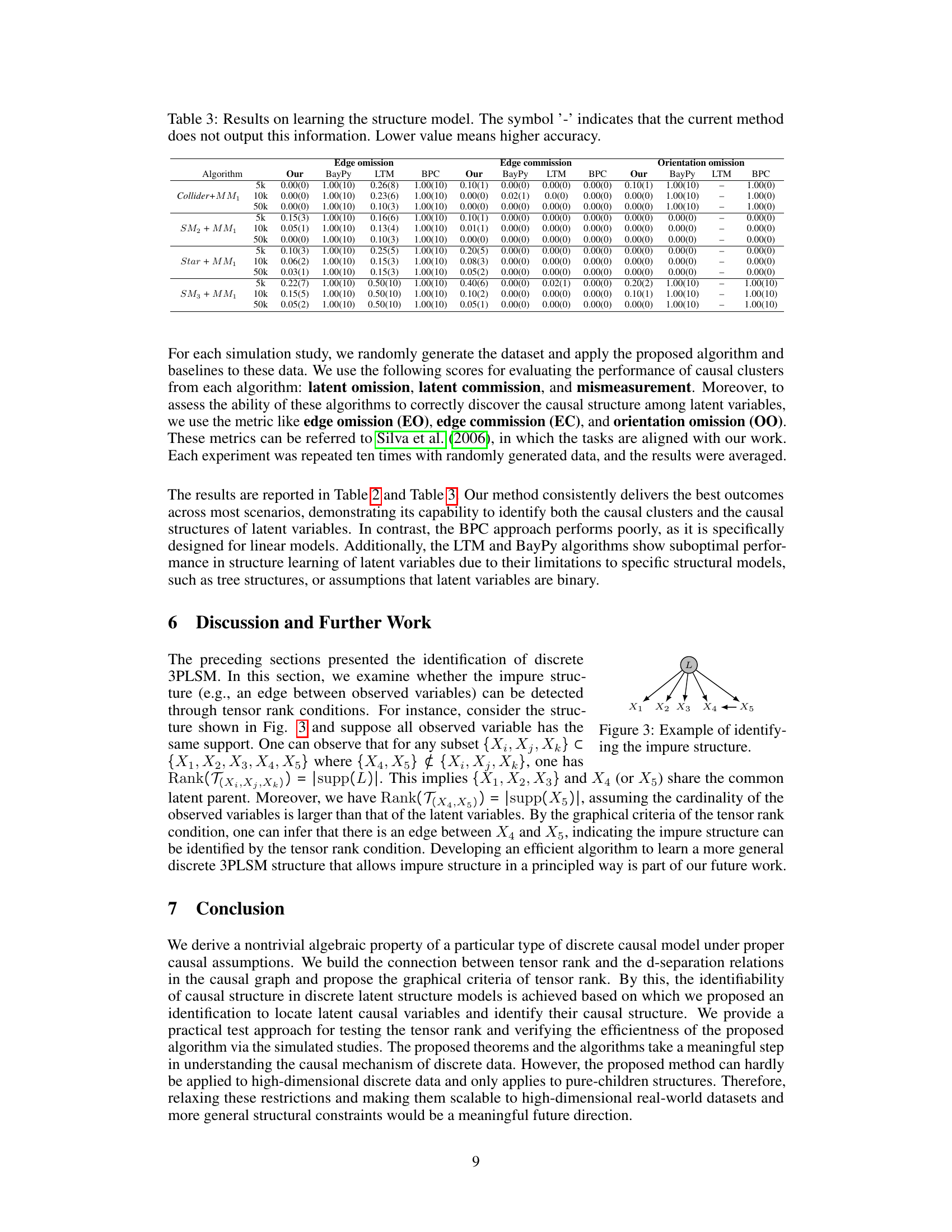
🔼 This table presents the results of experiments comparing four different algorithms (Ours, BayPy, LTM, BPC) for learning pure measurement models in discrete data generated by the Discrete Latent Structure Model with Three-Pure Children (Discrete 3PLSM). The algorithms are evaluated based on three metrics: latent omission (the number of missing latents), latent commission (the number of false positive latents), and mismeasurements (the number of incorrectly measured variables). The data were generated with varying sample sizes (5k, 10k, 50k) and two different model types (SM1, SM2) with additional mismeasurement conditions.
read the caption
Table 2: Results on learning pure measurement models, where the data is generated by the discrete 3PLSM. Lower value means higher accuracy.

🔼 This table presents the results of experiments evaluating the performance of different algorithms in learning pure measurement models. The data used in the experiments were generated using the discrete 3PLSM model. The algorithms are compared on three metrics: latent omission, latent commission, and mismeasurement. Lower values for these metrics indicate better performance.
read the caption
Table 2: Results on learning pure measurement models, where the data is generated by the discrete 3PLSM. Lower value means higher accuracy.
🔼 This table presents the results of learning pure measurement models using four different algorithms: the proposed method, Bayesian Pyramid Model (BayPy), Latent Tree Model (LTM), and Building Pure Cluster (BPC). The data is generated using the discrete three-pure-children latent structure model (Discrete 3PLSM). The table shows the performance of each algorithm in terms of latent omission, latent commission, and mismeasurement across three different sample sizes (5k, 10k, and 50k) and two different model configurations (SM1 + MM1 and SM2 + MM1). Lower values indicate better accuracy. The results demonstrate the superior performance of the proposed method, particularly in scenarios with larger sample sizes.
read the caption
Table 2: Results on learning pure measurement models, where the data is generated by the discrete 3PLSM. Lower value means higher accuracy.

🔼 This table presents the results of experiments evaluating the performance of different algorithms in learning pure measurement models. The data for these experiments was generated using the discrete 3PLSM (three-pure children discrete latent structure model). The table shows the performance metrics for three different scenarios with varying sample sizes (5k, 10k, and 50k). The metrics used include latent omission, latent commission, and mismeasurements, reflecting the accuracy of the algorithms in correctly identifying the latent variables and their relationships with observed variables. Lower values indicate higher accuracy for all metrics.
read the caption
Table 2: Results on learning pure measurement models, where the data is generated by the discrete 3PLSM. Lower value means higher accuracy.

🔼 This table presents the results of evaluating different algorithms’ performance in learning pure measurement models. The data used for evaluation was generated using the discrete 3PLSM model. The algorithms compared are: Our method, BayPy, LTM, and BPC. The table shows the accuracy of each algorithm in three scenarios (5k, 10k, 50k samples), evaluating metrics of latent omission, latent commission, and mismeasurement. Lower scores indicate better performance. The results are categorized based on the specific structure and measurement models used in generating the data (SM1+MM1, SM2+MM1, SM3+MM1, SM2+MM2, SM3+MM2).
read the caption
Table 2: Results on learning pure measurement models, where the data is generated by the discrete 3PLSM. Lower value means higher accuracy.
Full paper#
