TL;DR#
Snapshot Compressive Imaging (SCI) aims to reconstruct high-dimensional data (like videos) from a single 2D measurement, but existing methods often require computationally intensive training or struggle with noisy data. The challenge is finding efficient algorithms that work well in various scenarios without needing substantial training data. Existing methods using Deep Neural Networks (DNNs) require extensive training data and struggle with generalization, while classic methods are limited to simpler structures and perform poorly with high-dimensional data.
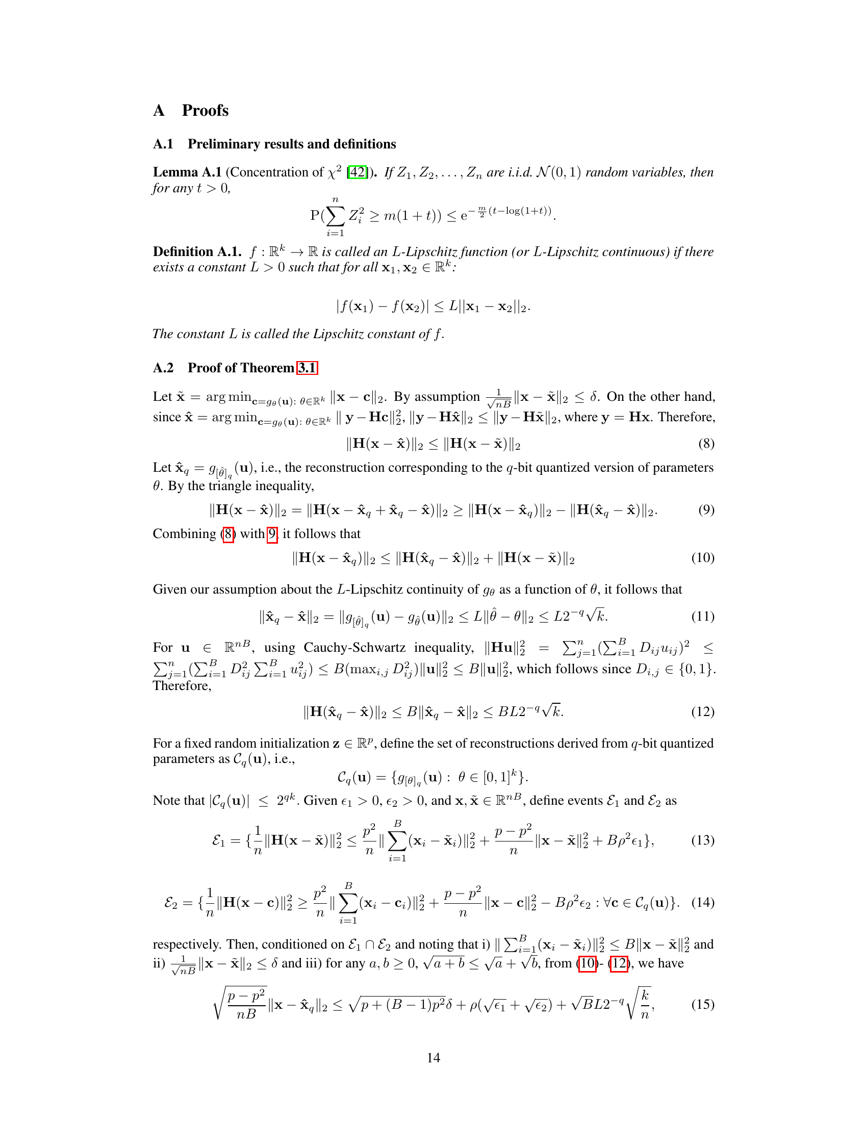
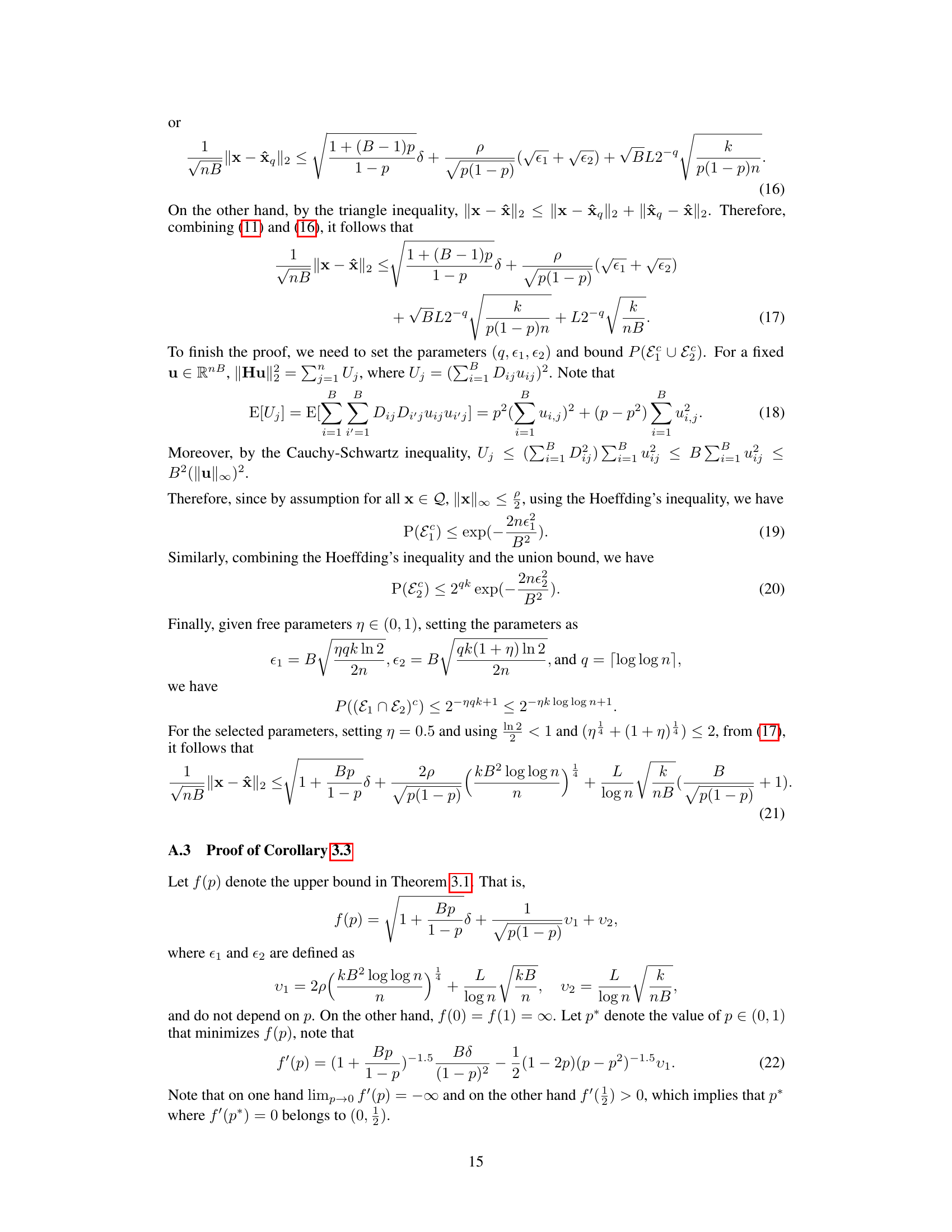
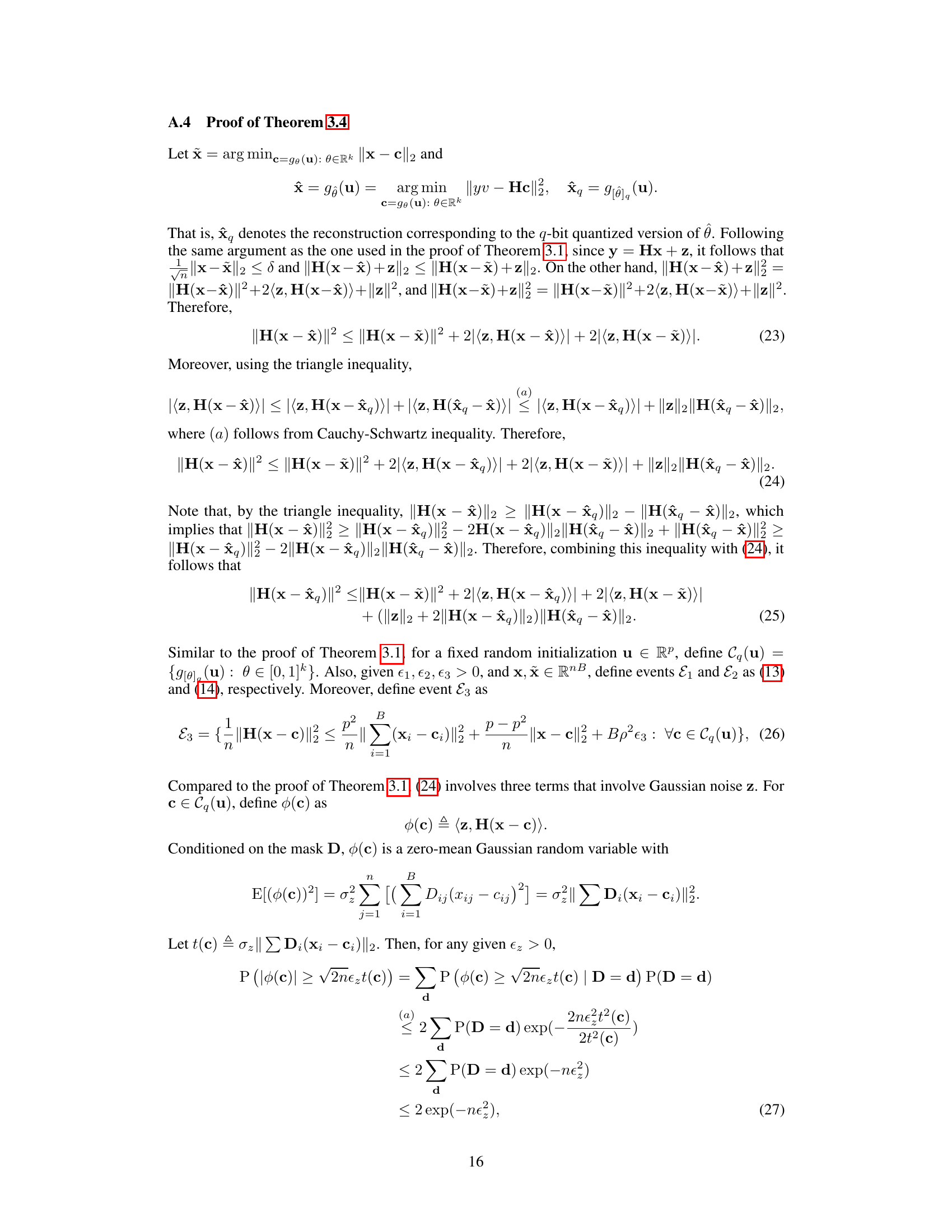
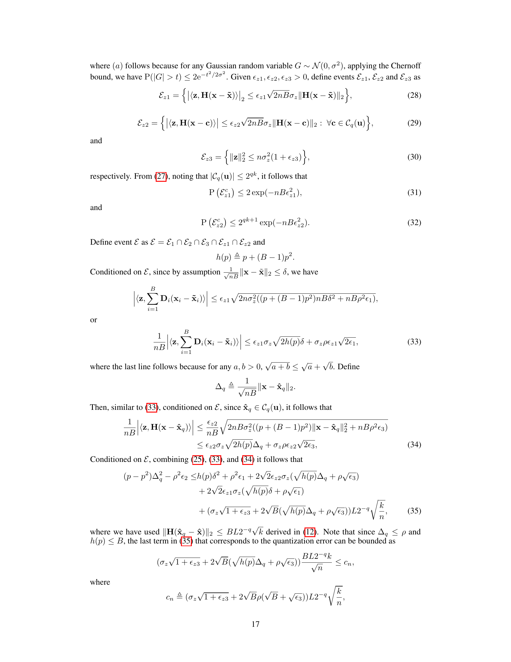
This research introduces a new method called SCI-BDVP, which uses untrained neural networks. SCI-BDVP employs a theoretical framework to optimize the image acquisition process and utilizes a technique called ‘bagged-DIP’ to improve robustness and performance, particularly when dealing with noise. Experiments show that SCI-BDVP surpasses other UNN-based methods for video SCI recovery, especially in the presence of noise. The proposed method also provides insights into how to best design the image acquisition masks, ultimately advancing the capabilities and efficiency of SCI.
Key Takeaways#
Why does it matter?#
This paper is crucial for researchers in computational imaging and deep learning. It offers a novel theoretical framework for understanding untrained neural network (UNN)-based snapshot compressive imaging (SCI), directly impacting the design of optimized masks and enhancing recovery performance. The introduction of SCI-BDVP, achieving state-of-the-art results, opens new avenues for UNN-based inverse problem solutions and further research in UNN theory. Its practical implications in video and hyperspectral imaging are significant, providing faster and more efficient imaging solutions.
Visual Insights#

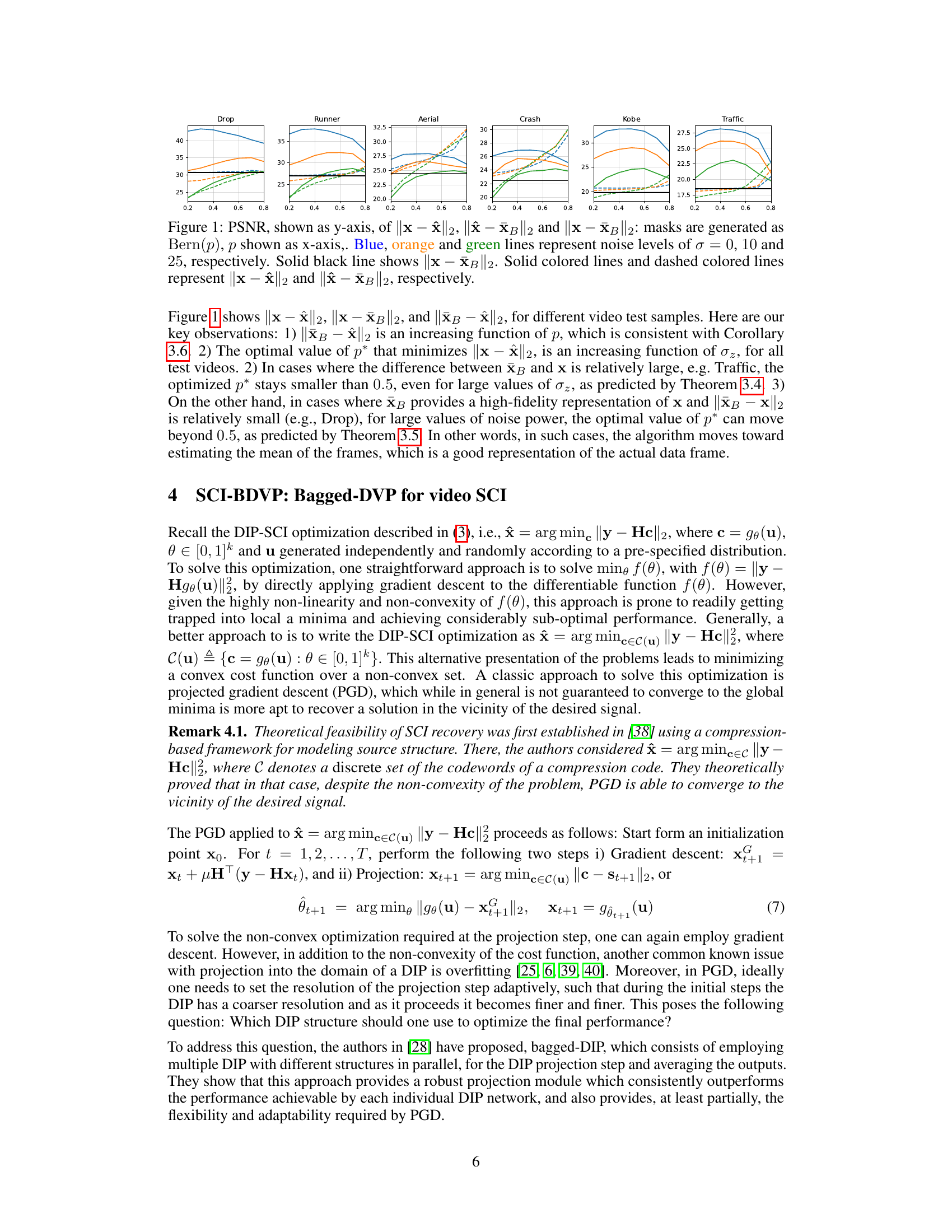
🔼 This figure shows the PSNR (Peak Signal-to-Noise Ratio) values for different metrics related to the reconstruction error, plotted against the probability (p) of a mask entry being non-zero. Different colored lines represent different levels of added noise (sigma = 0, 10, and 25). It illustrates how the reconstruction error changes with varying mask sparsity (p) and noise levels. The results help to determine the optimal mask sparsity for different noise conditions.
read the caption
Figure 1: PSNR, shown as y-axis, of ||x - ✰||2, ||✰ - XB||2 and ||x - XB||2: masks are generated as Bern(p), p shown as x-axis,. Blue, orange and green lines represent noise levels of σ = 0, 10 and 25, respectively. Solid black line shows ||x - XB||2. Solid colored lines and dashed colored lines represent ||x - ✰||2 and ||✰ - XB||2, respectively.

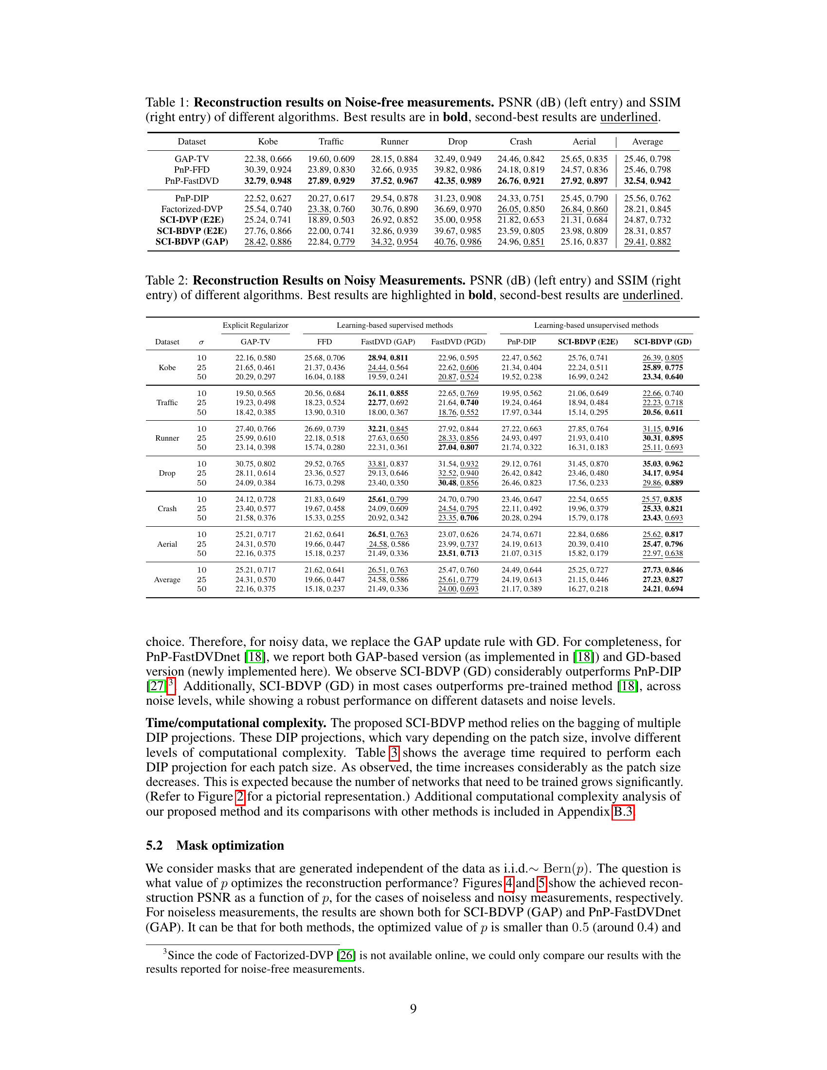
🔼 This table presents a comparison of different algorithms for snapshot compressive imaging (SCI) reconstruction on noise-free measurements. It shows the Peak Signal-to-Noise Ratio (PSNR) and Structural Similarity Index (SSIM) for each algorithm across various datasets (Kobe, Traffic, Runner, Drop, Crash, Aerial). The best and second-best results are highlighted for easy comparison.
read the caption
Table 1: Reconstruction results on Noise-free measurements. PSNR (dB) (left entry) and SSIM (right entry) of different algorithms. Best results are in bold, second-best results are underlined.
In-depth insights#
SCI’s UNN Approach#
The research paper explores Snapshot Compressive Imaging (SCI) recovery using untrained neural networks (UNNs), offering a unique approach that avoids the computationally expensive retraining needed for different source models and measurement scenarios. This UNN-based method leverages the power of UNNs to model source structure effectively, even without prior training data. The study presents both a theoretical framework to optimize the performance and design of data-modulating masks and algorithmic innovations such as SCI Bagged Deep Video Prior (SCI-BDVP), which addresses the common challenges faced by standard UNN solutions. SCI-BDVP shows state-of-the-art performance, particularly in scenarios with noisy measurements, outperforming even supervised methods. The theoretical findings establish a connection between recoverable data frames and UNN parameters, further refining mask optimization strategies. Overall, this approach offers a promising avenue for developing efficient and robust SCI recovery techniques.
Theoretical SCI Mask#
A theoretical analysis of snapshot compressive imaging (SCI) masks could offer invaluable insights. It would move beyond empirical mask design, allowing for principled optimization based on fundamental properties of the imaging system and the underlying signal. Such a theoretical framework could address the trade-offs between mask sparsity, measurement efficiency, and reconstruction quality. Key parameters like the probability of a mask entry being nonzero and its spatial distribution are ripe for theoretical analysis. Understanding how these parameters affect the conditioning of the sensing matrix would be crucial. A strong theoretical foundation would also guide the development of novel mask patterns optimized for specific signal types (e.g., videos or hyperspectral images) or noise conditions, leading to improved recovery algorithms. Exploring the relationship between mask design and reconstruction complexity in different algorithms would be essential for guiding real-world implementations. This theoretical approach could also potentially lead to the development of hardware-aware masks, optimized for specific sensor capabilities and computational constraints. By providing a rigorous mathematical understanding of SCI masks, this approach paves the way for significantly enhanced SCI system design and reconstruction capabilities.
SCI-BDVP Algorithm#
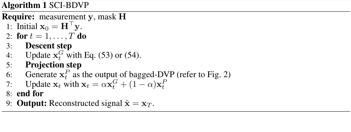
The SCI-BDVP algorithm tackles snapshot compressive imaging (SCI) recovery by leveraging the power of bagged deep video priors (BDVPs). Unlike traditional DIP methods prone to local minima and overfitting, SCI-BDVP employs multiple DVPs, each operating at a different scale (patch size), to achieve robust reconstruction. The algorithm integrates a gradient descent step, combined with a bagged projection that averages the outputs of the diverse DVPs, mitigating overfitting and enhancing robustness. A key advantage is its unsupervised nature, eliminating the need for extensive training data. This is particularly beneficial for SCI applications where diverse datasets and varying noise levels may hinder the generalizability of supervised methods. The use of a skip connection that combines gradient descent and bagged-DVP outputs further enhances performance. Experimental results show SCI-BDVP achieving state-of-the-art performance, especially in noisy conditions, surpassing both supervised and other UNN-based techniques. The theoretical framework provided in the paper helps optimize mask parameters for improved recovery, leading to significant advancements in the field of SCI.
Bagged-DIP for SCI#
The concept of “Bagged-DIP for SCI” introduces a novel approach to snapshot compressive imaging (SCI) by leveraging the strengths of the Bagged-Deep-Image-Prior (Bagged-DIP) technique. Bagged-DIP addresses limitations of traditional DIP methods, which often suffer from overfitting and sensitivity to initialization. By training multiple DIPs independently on various subsets of the data and averaging their predictions, Bagged-DIP enhances robustness and generalization. In the context of SCI, this translates to improved reconstruction of high-dimensional data cubes from a single 2D measurement, even under noisy conditions. The method’s effectiveness lies in its ability to capture complex source structures without extensive training data, making it suitable for diverse SCI applications. Theoretical analysis helps optimize parameters like mask design, further enhancing the performance of the algorithm. The integration of Bagged-DIP into SCI recovery algorithms offers a promising direction for advancing computational imaging. The results demonstrate state-of-the-art performance against existing methods. It’s especially beneficial for video and hyperspectral imaging where high-dimensional data requires computationally efficient recovery techniques.
Future Research#
Future research directions stemming from this work on untrained neural networks (UNNs) for snapshot compressive imaging (SCI) could explore several promising avenues. Firstly, a deeper theoretical analysis of UNN performance under various mask designs and noise models is crucial. While the paper provides a foundation, extending this work to more complex, non-i.i.d. mask structures commonly used in practical SCI systems is vital. Secondly, the optimization of the proposed SCI-BDVP algorithm itself offers opportunities; the algorithm’s parameters (e.g., the averaging coefficient) can be further refined through more extensive empirical analysis and theoretical justification. Thirdly, applying the bagged-DIP concept to other inverse problems beyond SCI could reveal its broader applicability and potential benefits. Finally, extending the work to address the challenges of hyperspectral imaging, where the spectral dimension adds significant complexity, represents a major opportunity for advancement in this field. Investigating the effect of various data-modulating masks in HSI and exploring novel theoretical bounds on recovery performance within this more challenging context would significantly advance the state-of-the-art.
More visual insights#
More on figures

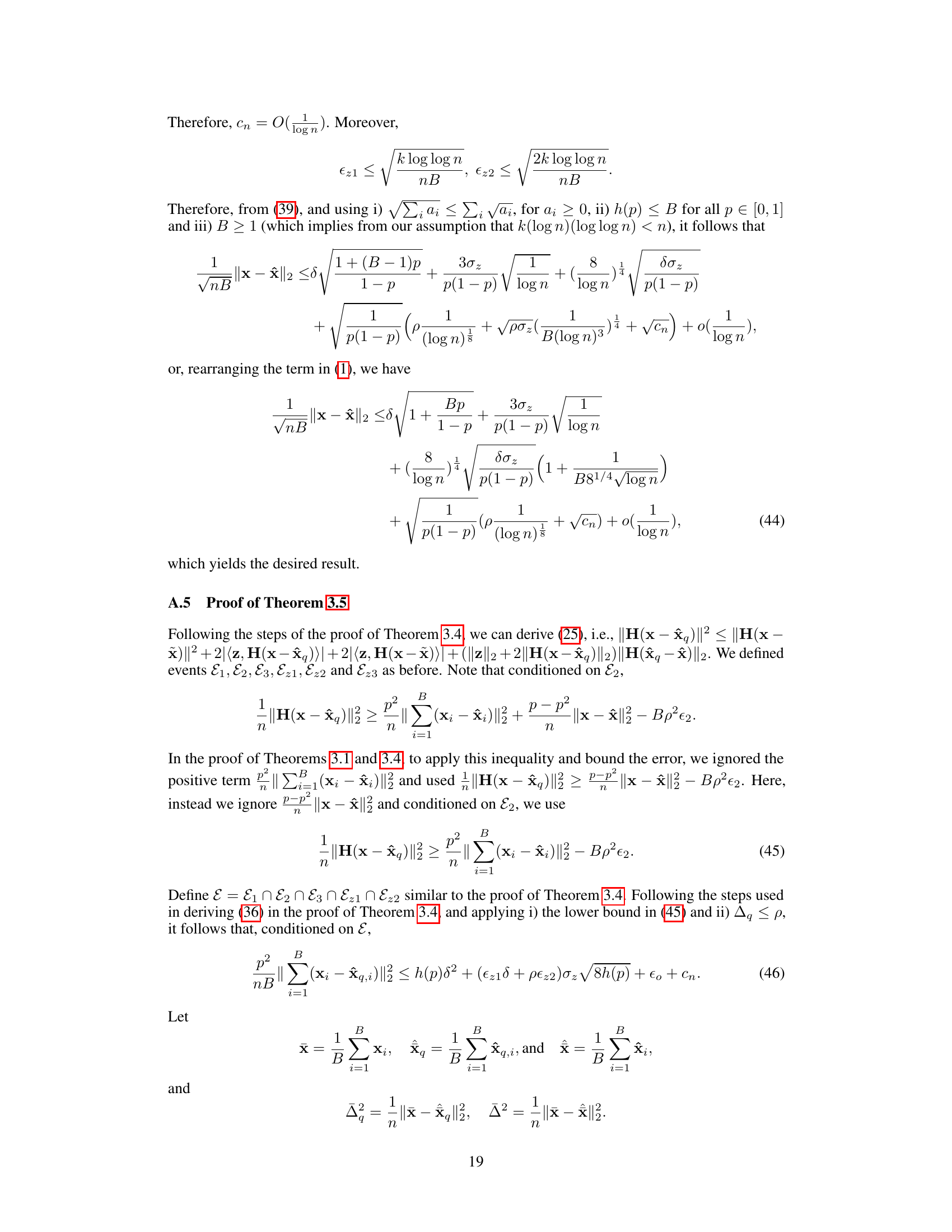
🔼 This figure illustrates the architecture of the SCI-BDVP algorithm. It uses K separate DIP (Deep Image Prior) blocks, each operating on a different patch size of the input video data. The outputs of these DIP blocks are averaged (blue dot) and combined with a gradient descent result (red lines and orange dot) to form an estimate. This process is repeated K times. The overall algorithm leverages a weighted average of the gradient descent step and the bagged DIP output (fusion), using the 2D measurement (y) and the 3D mask (H) for training the DIPs. The objective is to reconstruct a high-dimensional 3D data cube from a single 2D measurement.
read the caption
Figure 2: The structure of SCI-BDVP. There are K estimates generated, each using a different patch size. The blue dot denotes averaging the K estimates, the orange dot denotes averaging x and x with weight a, the red dot denotes the loss function used for training the DIP parameters, requiring xf, y and H. The red lines denote using 3D gradient descent result xf, which is used for training the parameters of the k-th DIP (red dot), and averaging with projection output xf (orange dot). The green lines denote using 2D measurement y and 3D binary mask H for training parameters of DIPs in different estimate k.
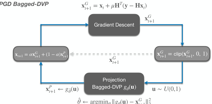
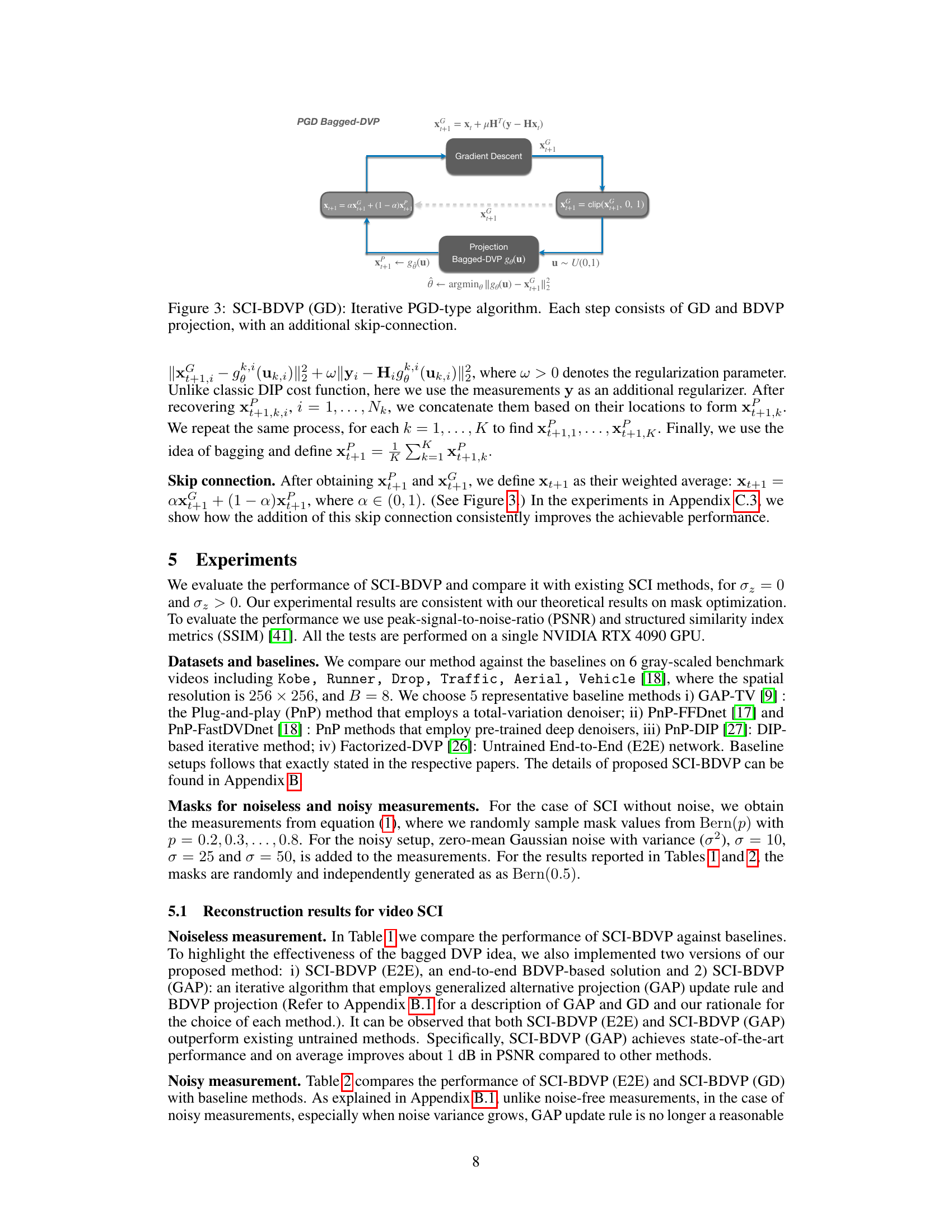
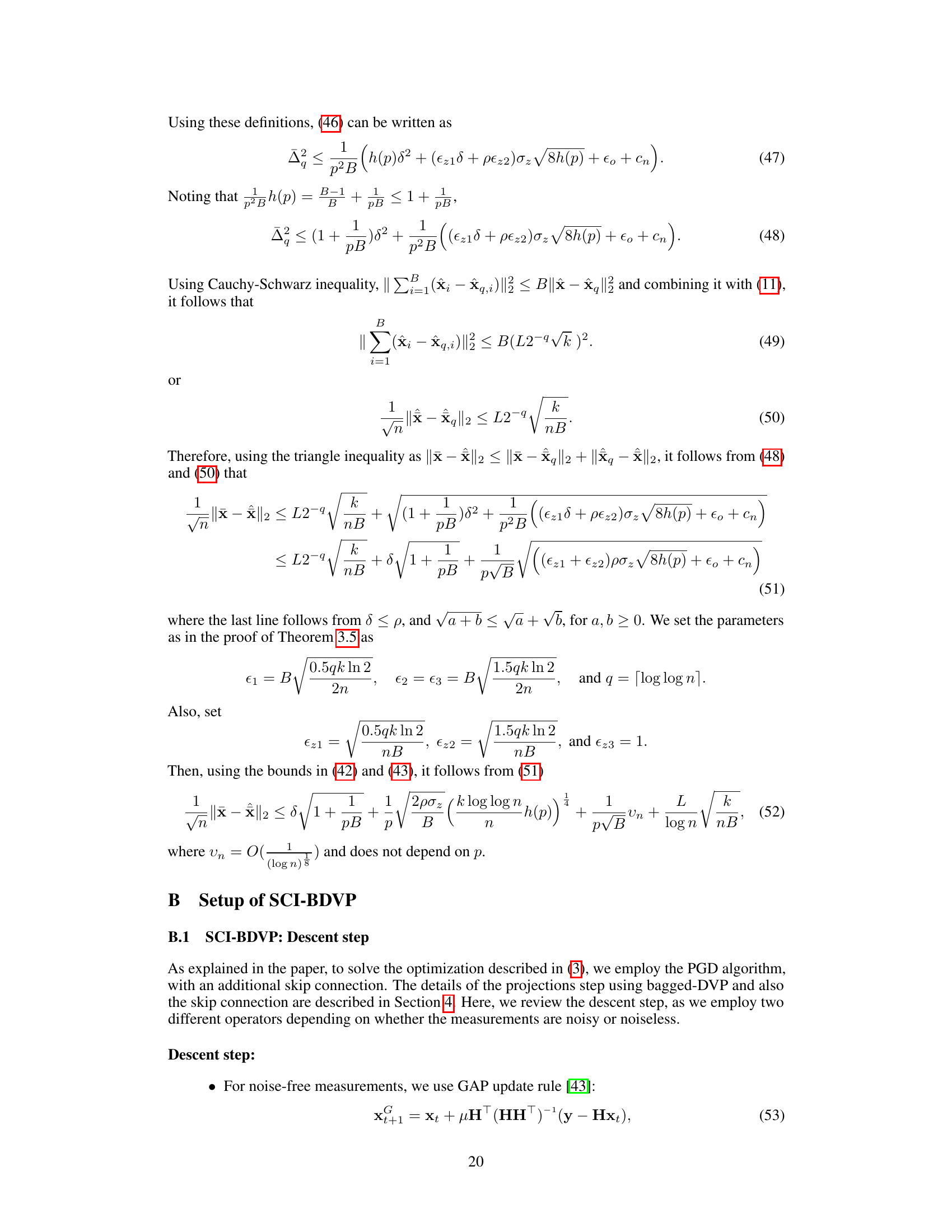
🔼 This figure shows the iterative process of the proposed SCI-BDVP algorithm. Each iteration involves two main steps: gradient descent (GD) to update the estimate, and projection onto the domain of a bagged deep video prior (BDVP). The BDVP uses multiple deep image priors operating at different scales, which helps to address the issues of overfitting and local minima that are often encountered in DIP-based methods. Finally, a skip connection combines the results from GD and BDVP, further improving performance.
read the caption
Figure 3: SCI-BDVP (GD): Iterative PGD-type algorithm. Each step consists of GD and BDVP projection, with an additional skip-connection.

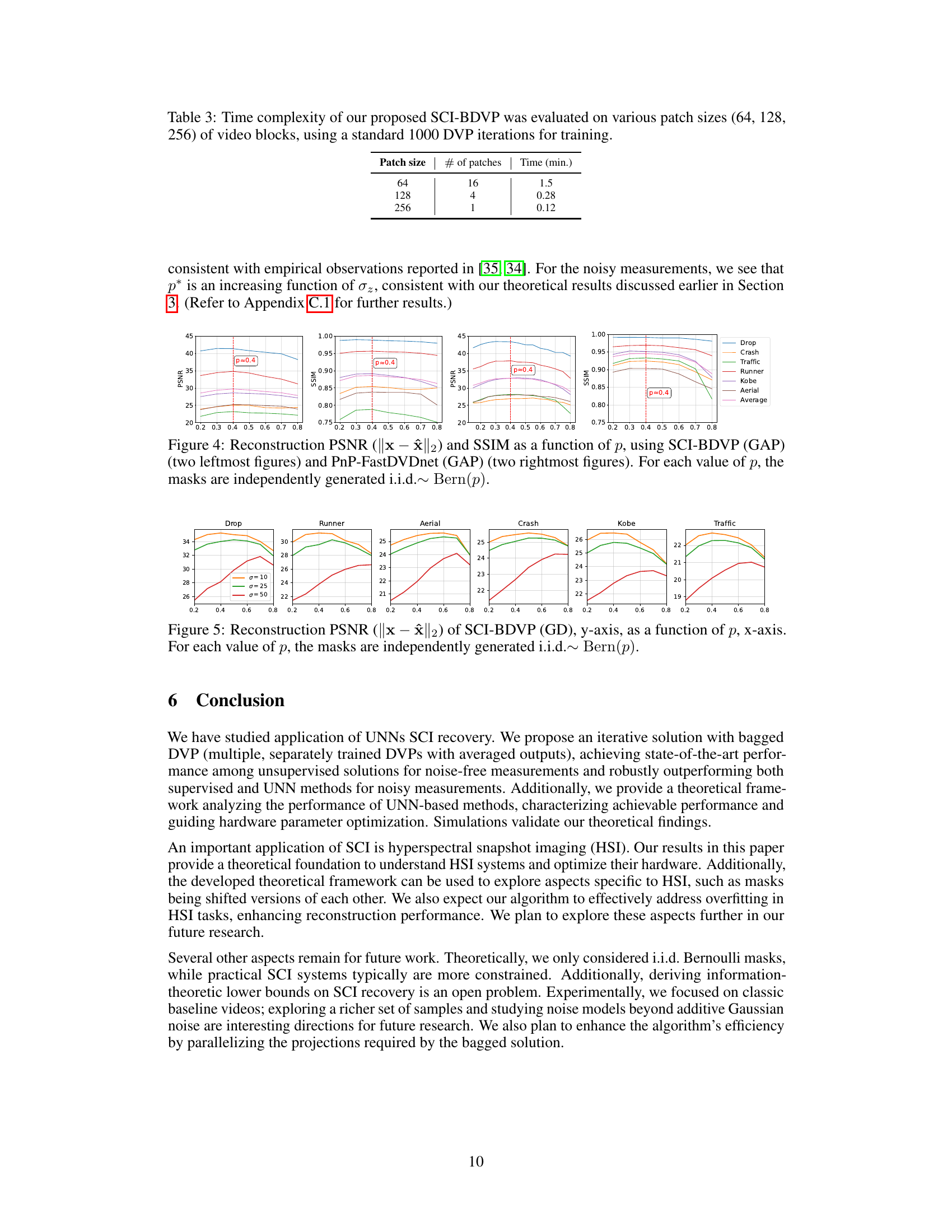
🔼 This figure displays the PSNR (Peak Signal-to-Noise Ratio) for different metrics as a function of the non-zero probability (p) of the mask. It illustrates how reconstruction error changes depending on the mask and noise levels. The different colored lines represent different noise levels, showing the impact of noise on the reconstruction quality and its relation to the mask’s probability parameter (p).
read the caption
Figure 1: PSNR, shown as y-axis, of ||x - ✰||2, ||✰ - XB||2 and ||x - XB||2: masks are generated as Bern(p), p shown as x-axis,. Blue, orange and green lines represent noise levels of σ = 0, 10 and 25, respectively. Solid black line shows ||x - XB||2. Solid colored lines and dashed colored lines represent ||x - ✰||2 and ||✰ - XB||2, respectively.

🔼 The figure displays the PSNR (Peak Signal-to-Noise Ratio) for different video samples, plotted against the probability (p) of a mask entry being non-zero. Different colored lines represent different noise levels (σ = 0, 10, 25). The plot shows the impact of mask probability (p) and noise on the reconstruction error, comparing the overall error (||x - ŷ||2) with the errors due to DIP representation limitations (||ŷ - xB||2) and the deviation from the average frame (||x - xB||2).
read the caption
Figure 1: PSNR, shown as y-axis, of ||x - ŷ||2, ||ŷ - xB||2 and ||x - xB||2: masks are generated as Bern(p), p shown as x-axis,. Blue, orange and green lines represent noise levels of σ = 0, 10 and 25, respectively. Solid black line shows ||x - xB||2. Solid colored lines and dashed colored lines represent ||x - ŷ||2 and ||ŷ - xB||2, respectively.
🔼 This figure shows the PSNR (Peak Signal-to-Noise Ratio) for three different metrics of reconstruction error as a function of the probability p of generating binary masks using a Bernoulli distribution. It demonstrates how the optimal probability p* changes with increasing noise levels (σ = 0, 10, and 25) for different video samples. The three metrics represented are the error between the original and reconstructed signals (||x - ˆx||2), the error between the reconstructed signal and the average of all frames (||ˆx - xB||2), and the error between the average of the frames and the original (||x - xB||2).
read the caption
Figure 1: PSNR, shown as y-axis, of ||x - ˆx||2, ||ˆx - xB||2 and ||x - xB||2: masks are generated as Bern(p), p shown as x-axis,. Blue, orange and green lines represent noise levels of σ = 0, 10 and 25, respectively. Solid black line shows ||x - xB||2. Solid colored lines and dashed colored lines represent ||x - ˆx||2 and ||ˆx - xB||2, respectively.

🔼 This figure shows the detailed network architecture of the Deep Video Prior (DVP) used in the SCI-BDVP algorithm. It consists of three DVP blocks, each composed of a 2D Convolution (Conv) layer with a kernel size of 3, a ReLU activation function, and an Upsample layer with a scaling factor of 2. The final Video Output Block contains a 2D Convolution layer with a kernel size of 3 and a Sigmoid activation function. Each DVP block has 128 input and output channels, while the output block’s output channels match the dimensions of the video frame. This design aims to efficiently capture and reconstruct video data at different scales.
read the caption
Figure 6: Network structure of DVP we use in SCI-BDVP.

🔼 This figure displays the PSNR (Peak Signal-to-Noise Ratio) for different video test samples, illustrating the impact of mask probability (p) and noise level (σ) on reconstruction error. The three different error metrics presented show the trade-offs between approximating the true signal (x), the mean frame (XB), and the reconstruction (✰).
read the caption
Figure 1: PSNR, shown as y-axis, of ||x - ✰||2, ||✰ - XB||2 and ||x - XB||2: masks are generated as Bern(p), p shown as x-axis,. Blue, orange and green lines represent noise levels of σ = 0, 10 and 25, respectively. Solid black line shows ||x - XB||2. Solid colored lines and dashed colored lines represent ||x - ✰||2 and ||✰ - XB||2, respectively.

🔼 This figure shows the Peak Signal-to-Noise Ratio (PSNR) for different video samples with varying mask probabilities (p) and noise levels. It compares three different error metrics: ||x - ✰||2 (reconstruction error), ||✰ - XB||2 (error of the mean frame approximation), and ||x - XB||2 (error between the original video and the mean frame). The results illustrate how the optimal mask probability (p) and the relationship between the different error metrics change with varying noise levels.
read the caption
Figure 1: PSNR, shown as y-axis, of ||x - ✰||2, ||✰ - XB||2 and ||x - XB||2: masks are generated as Bern(p), p shown as x-axis,. Blue, orange and green lines represent noise levels of σ = 0, 10 and 25, respectively. Solid black line shows ||x - XB||2. Solid colored lines and dashed colored lines represent ||x - ✰||2 and ||✰ - XB||2, respectively.
🔼 The figure shows the PSNR (Peak Signal-to-Noise Ratio) for three different error metrics: ||x - ✰||2, ||✰ - XB||2, and ||x - XB||2, plotted against different values of p (probability of a mask entry being non-zero). The lines are color-coded to represent different noise levels (σ = 0, 10, and 25). The plot illustrates how the optimal value of p changes with increasing noise levels and how the different error metrics behave under varying mask sparsity and noise conditions.
read the caption
Figure 1: PSNR, shown as y-axis, of ||x - ✰||2, ||✰ - XB||2 and ||x - XB||2: masks are generated as Bern(p), p shown as x-axis,. Blue, orange and green lines represent noise levels of σ = 0, 10 and 25, respectively. Solid black line shows ||x - XB||2. Solid colored lines and dashed colored lines represent ||x - ✰||2 and ||✰ - XB||2, respectively.
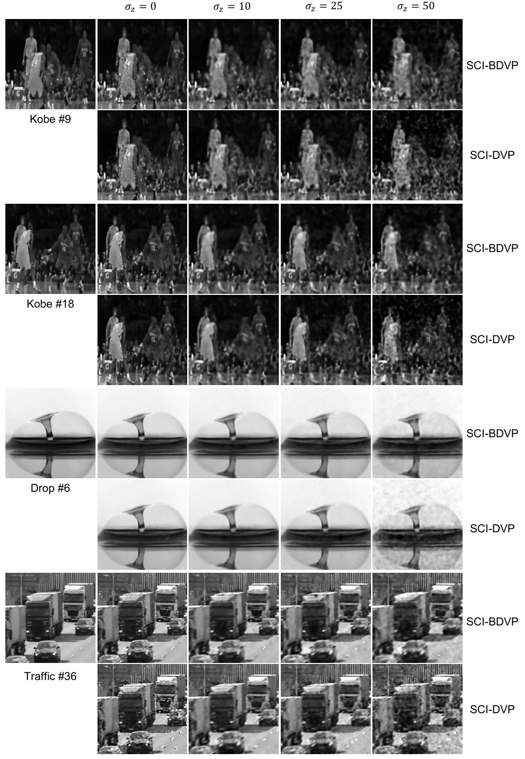
🔼 This figure compares the reconstruction results of SCI-BDVP and SCI-DVP methods on four different video samples at four different noise levels (σz = 0, 10, 25, 50). The leftmost column shows the original clean frames. The remaining columns illustrate reconstructions for each method and noise level. The results visually demonstrate the improved performance of SCI-BDVP, particularly in higher noise levels.
read the caption
Figure 10: Reconstruction results of SCI-BDVP vs. SCI-DVP. (leftmost images are clean frames).

🔼 This figure compares the reconstruction results of SCI-BDVP and SCI-DVP methods for several video sequences under different noise levels (σz = 0, 10, 25, 50). The leftmost column shows the original clean frames. Each row represents a different video sequence, and each column displays the reconstruction for a specific noise level. By visually comparing the results, one can assess the relative performance of the two methods in handling noisy measurements.
read the caption
Figure 10: Reconstruction results of SCI-BDVP vs. SCI-DVP. (leftmost images are clean frames).

🔼 The figure shows the Peak Signal-to-Noise Ratio (PSNR) for different video test samples, as a function of the probability (p) of a mask entry being non-zero. The PSNR is calculated in three ways: the difference between the reconstructed video and the true video (||x - ŷ||2), the difference between the reconstructed video and the average frame (||ŷ - xB||2), and the difference between the average frame and the true video (||x - xB||2). Different colored lines represent different noise levels (σ = 0, 10, and 25). This illustrates the relationship between mask generation and reconstruction error, especially considering noise.
read the caption
Figure 1: PSNR, shown as y-axis, of ||x - ŷ||2, ||ŷ - xB||2 and ||x - xB||2: masks are generated as Bern(p), p shown as x-axis,. Blue, orange and green lines represent noise levels of σ = 0, 10 and 25, respectively. Solid black line shows ||x - xB||2. Solid colored lines and dashed colored lines represent ||x - ŷ||2 and ||ŷ - xB||2, respectively.
🔼 The figure shows the Peak Signal-to-Noise Ratio (PSNR) of three different error terms: ||x - ✰||2, ||✰ - XB||2, and ||x - XB||2, plotted against the probability p of a mask entry being non-zero (Bernoulli distribution). Different colored lines represent different levels of noise (σ = 0, 10, and 25). The plot aims to illustrate the impact of mask design (controlled by p) on the reconstruction quality under varying noise conditions. It shows how the optimal probability p* changes with the level of noise in the measurements.
read the caption
Figure 1: PSNR, shown as y-axis, of ||x - ✰||2, ||✰ - XB||2 and ||x - XB||2: masks are generated as Bern(p), p shown as x-axis,. Blue, orange and green lines represent noise levels of σ = 0, 10 and 25, respectively. Solid black line shows ||x - XB||2. Solid colored lines and dashed colored lines represent ||x - ✰||2 and ||✰ - XB||2, respectively.
More on tables
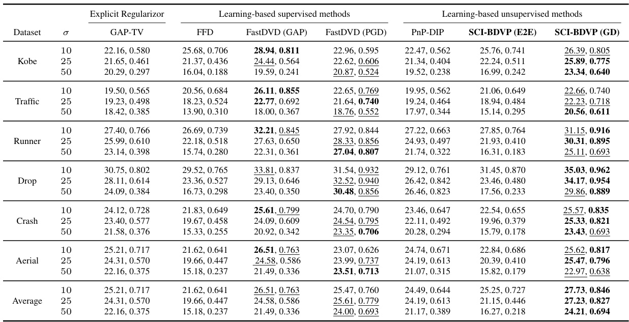
🔼 This table presents the reconstruction results on noisy measurements for several algorithms, including GAP-TV, FFDNet, FastDVDNet, PnP-DIP, SCI-BDVP (E2E), and SCI-BDVP (GD). The results are shown for different noise levels (σ = 10, 25, 50) and for several video datasets (Kobe, Traffic, Runner, Drop, Crash, Aerial). PSNR (Peak Signal-to-Noise Ratio) and SSIM (Structural Similarity Index) are used as evaluation metrics. The best and second-best results for each dataset and noise level are highlighted in bold and underlined, respectively.
read the caption
Table 2: Reconstruction Results on Noisy Measurements. PSNR (dB) (left entry) and SSIM (right entry) of different algorithms. Best results are highlighted in bold, second-best results are underlined.

🔼 This table shows the time it takes to train the SCI-BDVP model for different patch sizes. The time increases as the patch size decreases because more networks need to be trained.
read the caption
Table 3: Time complexity of our proposed SCI-BDVP was evaluated on various patch sizes (64, 128, 256) of video blocks, using a standard 1000 DVP iterations for training.

🔼 This table shows the number of inner and outer iterations used for training the SCI-BDVP model for different datasets (Kobe, Traffic, Runner, Drop, Crash, Aerial) and for different patch sizes (64, 128, 256 pixels). It also differentiates between the training for noise-free and noisy measurements. The inner iterations represent iterations within each patch size for DIP training, while the outer iterations represent the number of times the overall PGD optimization is performed.
read the caption
Table 4: Number of inner and outer iterations for training SCI-BDVP for different datasets and different estimates.

🔼 This table compares the computational time complexity of different methods (PnP-DIP, Factorized-DVP, Simple-DVP(E2E), and SCI-BDVP) for processing a single 8-frame video block. The results are categorized by whether noise is present in the measurement.
read the caption
Table 5: Time complexity over different methods on one 8-frame benchmark video block.

🔼 This table shows the impact of mask optimization on the reconstruction performance of SCI-BDVP for different videos and noise levels. It compares the PSNR and SSIM values obtained using a fixed regular binary mask (Bern(0.5)) against those obtained using an optimized mask. The results are broken down by noise level (σ = 0, 10, 25, 50) and whether the regular or optimized mask was used.
read the caption
Table 6: Detailed mask optimization effect on reconstruction with SCI-BDVP. PSNR (dB) (left entry) and SSIM (right entry) of the reconstruction results on different videos. (Reg.) represent reconstruction on using fixed regular binary mask, Dij ~ Bern(0.5). (OPT.) represents model tested on fixed optimized mask.
Full paper#
