TL;DR#
Causal structure learning, crucial in many fields, often struggles with designing effective interventions, especially when likelihood calculations are infeasible. Existing methods are often computationally expensive or limited by their assumptions. This paper tackles these challenges.
The proposed method, Causal Amortized Active Structure Learning (CAASL), utilizes a transformer-based network trained with reinforcement learning to directly predict the next intervention. This amortized approach bypasses the need for explicit likelihood computations and achieves impressive results on both synthetic and real-world single-cell gene expression data. CAASL successfully generalizes to new environments and intervention types, showcasing its potential for practical applications in various scientific domains.
Key Takeaways#
Why does it matter?#
This paper is important because it presents CAASL, a novel method for active intervention design in causal structure learning that does not require access to the likelihood, a major limitation in many real-world applications. Its amortized approach using deep reinforcement learning makes it efficient and generalizable, opening new avenues for research in causal inference, especially in complex domains like single-cell biology where likelihoods are often intractable. The demonstrated zero-shot generalization to different environments and intervention types further enhances its practicality and impact.
Visual Insights#
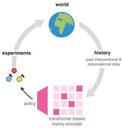
🔼 This figure illustrates the CAASL method, showing how the policy interacts with the world and history to make decisions. The world represents the environment under study. History comprises the past interventional and observational data, encoding information on previous experiments. The policy (a transformer-based history encoder) processes this data to suggest the next intervention. The experiments represent actions in the environment, such as gene knockouts or knockdowns.
read the caption
Figure 1: Causal Amortized Structure Learning (CAASL) is an active intervention design method that directly proposes the next intervention to perform by just a forward-pass of the transformer based policy.

🔼 This table lists the parameters used to simulate technical noise in single-cell RNA sequencing data for two different platforms: 10X Chromium and Drop-Seq. These parameters model various aspects of noise commonly encountered in scRNA-seq data, including outlier genes, library size effects, and dropouts. The values provided are used to generate realistic noise patterns in the simulated data for the experiments described in the paper.
read the caption
Table 1: Technical noise parameters for 10X Chromium and Drop-Seq Single-Cell RNA sequencing platforms that is used for experiments in this work.
In-depth insights#
Amortized Design#
Amortized design in this context refers to a machine learning approach that learns a single policy network to generate efficient intervention strategies for causal structure learning. Instead of repeatedly inferring a causal graph and then designing interventions (which is computationally expensive), the amortized policy directly predicts optimal interventions from observed data, thus achieving real-time, adaptive intervention design. This method offers significant computational savings and reduces the reliance on likelihood calculations, making it applicable to real-world scenarios where likelihoods are intractable. Generalization capabilities are another key advantage, with the ability to adapt to new environments and intervention types beyond those seen during training, suggesting practical usefulness in complex systems where distributional shifts are expected.
Reward Function#
The choice of reward function is crucial for the success of any reinforcement learning-based approach, and this paper’s design is no exception. The authors cleverly sidestep the challenge of likelihood-based reward functions, which are often intractable in real-world settings like gene regulatory network inference, by leveraging a pretrained likelihood-free amortized causal structure learning model (AVICI). This approach is elegant in its simplicity and efficiency, allowing for reward calculation without the computationally expensive steps of calculating likelihoods. The reward function is designed to directly measure the improvement in the accuracy of the causal graph estimate after each intervention. The authors thoughtfully address the challenge of reward design for causal discovery, where direct access to the ground truth causal structure is unavailable. The use of an amortized causal structure learning model enables the generation of a cheap yet effective reward function. This avoids iterative and slow computations typically associated with likelihood-based rewards. However, the reliance on an already trained AVICI model introduces a dependency that should be acknowledged. Future directions could explore more flexible approaches to defining reward functions, thereby reducing such dependencies.
Policy Network#
A policy network in the context of this research paper is a crucial component of the active intervention design process. Its core function is to learn an optimal strategy for selecting interventions in a causal structure learning setting. This network, which is trained using reinforcement learning, acts as a decision-maker. It receives the current state of the system (data acquired through past interventions) as input and outputs the next intervention to be performed. The choice of network architecture is significant; a transformer-based model is employed to effectively handle sequential data and encode design space symmetries. Crucially, the policy network’s learning is guided by a reward function. This function is designed to incentivize the selection of interventions that improve the quality of causal graph estimation. Therefore, the policy network learns to make decisions that not only are adaptive and real-time but also lead to more accurate inference of causal relationships, which highlights a strong focus on efficiency and sample-optimized learning.
Zero-Shot OOD#
The heading ‘Zero-Shot OOD’ likely refers to the model’s ability to generalize to out-of-distribution (OOD) scenarios without any prior training on those specific distributions. This is a significant aspect of the paper because it demonstrates the robustness and adaptability of the proposed method. A successful zero-shot OOD performance suggests that the learned representations have captured underlying causal mechanisms rather than simply memorizing the training data. The evaluation likely involved testing the model on various OOD datasets, each differing significantly from the training data in terms of the underlying causal graph structure, noise characteristics, or intervention types. The results section probably showcases how the model maintains good performance across diverse OOD environments, thus highlighting its ability to learn generalizable causal representations. This is a crucial finding since real-world applications often involve scenarios unseen during training, demanding robust, generalizable models.
SERGIO Testing#
SERGIO testing, within the context of evaluating an active intervention design policy for causal structure learning, is crucial for validating the policy’s performance and generalization capabilities in a realistic setting. The single-cell gene expression simulator, SERGIO, provides a complex and challenging environment due to inherent noise, missing data (often 70% or more), and the intricacies of gene regulatory networks. Effective SERGIO testing would involve evaluating the policy’s ability to learn causal relationships accurately under various conditions. This includes assessing performance across different graph structures, noise levels, and intervention types (gene knockouts and knockdowns). Zero-shot generalization is a critical aspect, examining the policy’s ability to adapt to unseen environments with varying dimensionalities or differing technical noise characteristics (simulating various scRNA-seq platforms). A rigorous evaluation must compare the policy’s performance against relevant baselines, such as random interventions or observational data collection, using established metrics like structural Hamming distance, AUPRC, and F1-score. The results from SERGIO testing would ultimately demonstrate the robustness and practical applicability of the learned policy for real-world causal discovery tasks in single-cell biology.
More visual insights#
More on figures
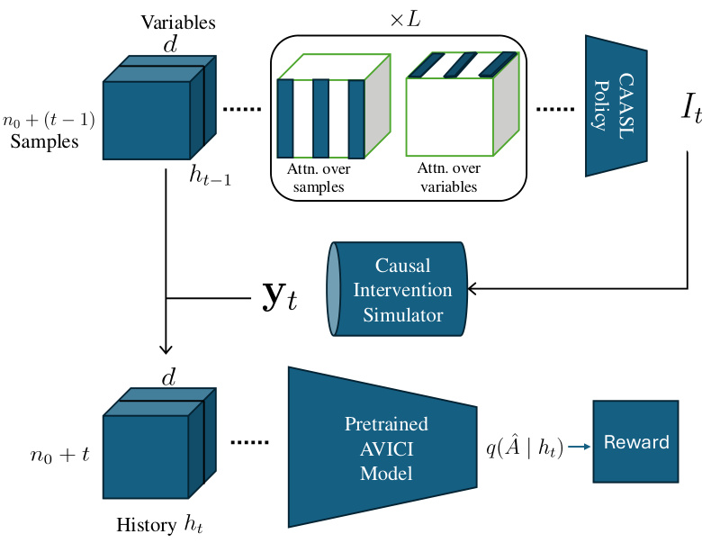
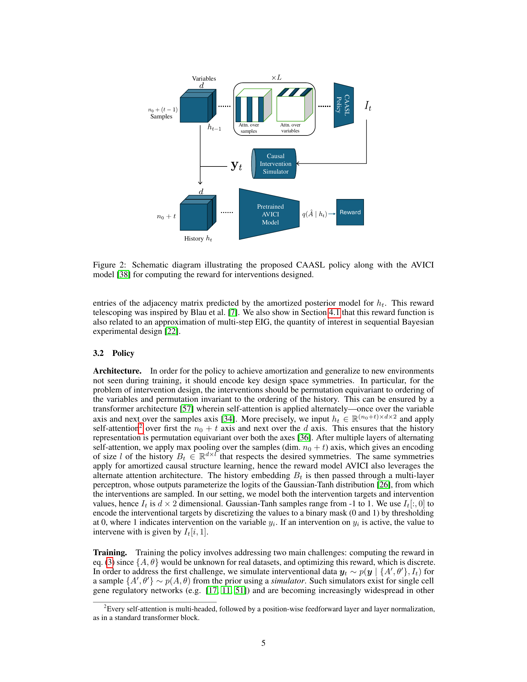
🔼 This figure shows a schematic diagram of the Causal Amortized Active Structure Learning (CAASL) policy. The CAASL policy takes the history of interventions and observations (ht−1) as input and uses a transformer network to generate the next intervention (It). The chosen intervention is then applied to a causal intervention simulator, which produces new observational data (yt). This new data, along with the previous history, is concatenated to form a new history (ht). This updated history is fed into a pretrained AVICI model, which estimates the posterior distribution q(Â|ht) over causal graphs. Finally, the reward is computed based on how well this posterior matches the true causal graph, providing feedback for training the CAASL policy via reinforcement learning.
read the caption
Figure 2: Schematic diagram illustrating the proposed CAASL policy along with the AVICI model [38] for computing the reward for interventions designed.
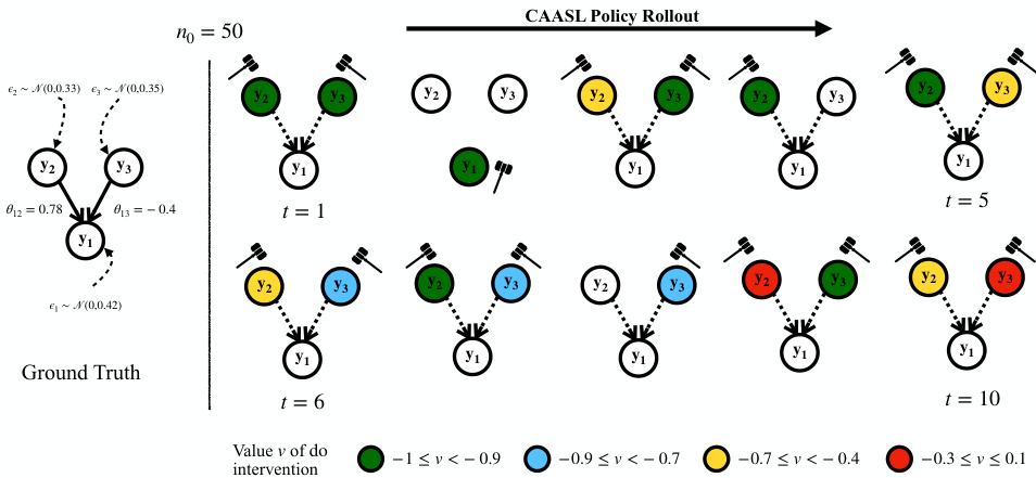
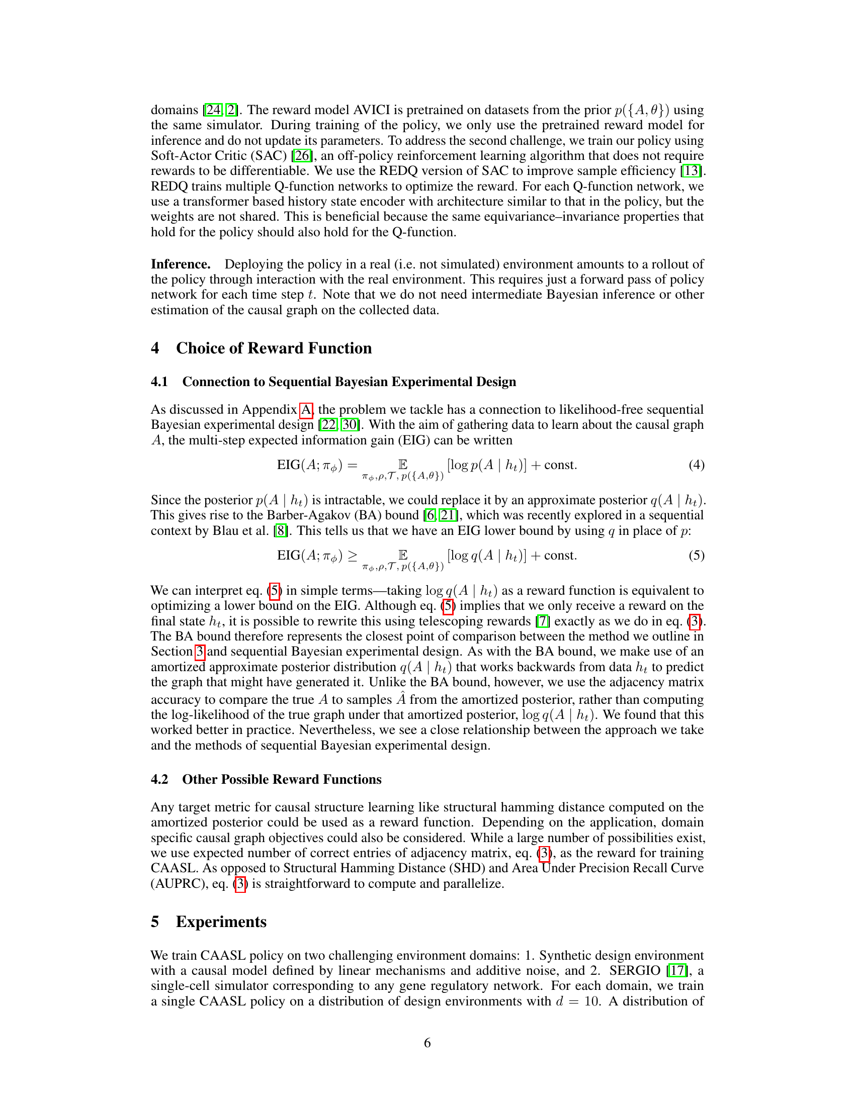
🔼 This figure visualizes a rollout of the trained CAASL policy on a random environment. The policy selects interventions targeting variables with children in the ground truth graph, initially exhibiting exploratory target selection and exploitative value selection, a trend which reverses as the episode progresses. The training environments had dimension d=2, hence the policy’s interaction with a d=3 environment is a zero-shot generalization task.
read the caption
Figure 3: Visualization of the rollout of the trained CAASL policy on a randomly sampled environment with n0 = 50 initial observational samples. Colored circles indicate nodes with a do intervention. The policy selects interventions that mostly correspond to the variables with a child in the ground truth graph. At t = 2, the policy selects the only child y1, which breaks all direct causal effects. This gives lesser information about the overall causal model. After this, y1 is never chosen. Initially, the policy is exploratory wrt targets and exploitative wrt values. This trend is reversed as the episode progresses. The policy is trained on environments with d = 2, therefore it has not seen any graphs with d = 3 before.

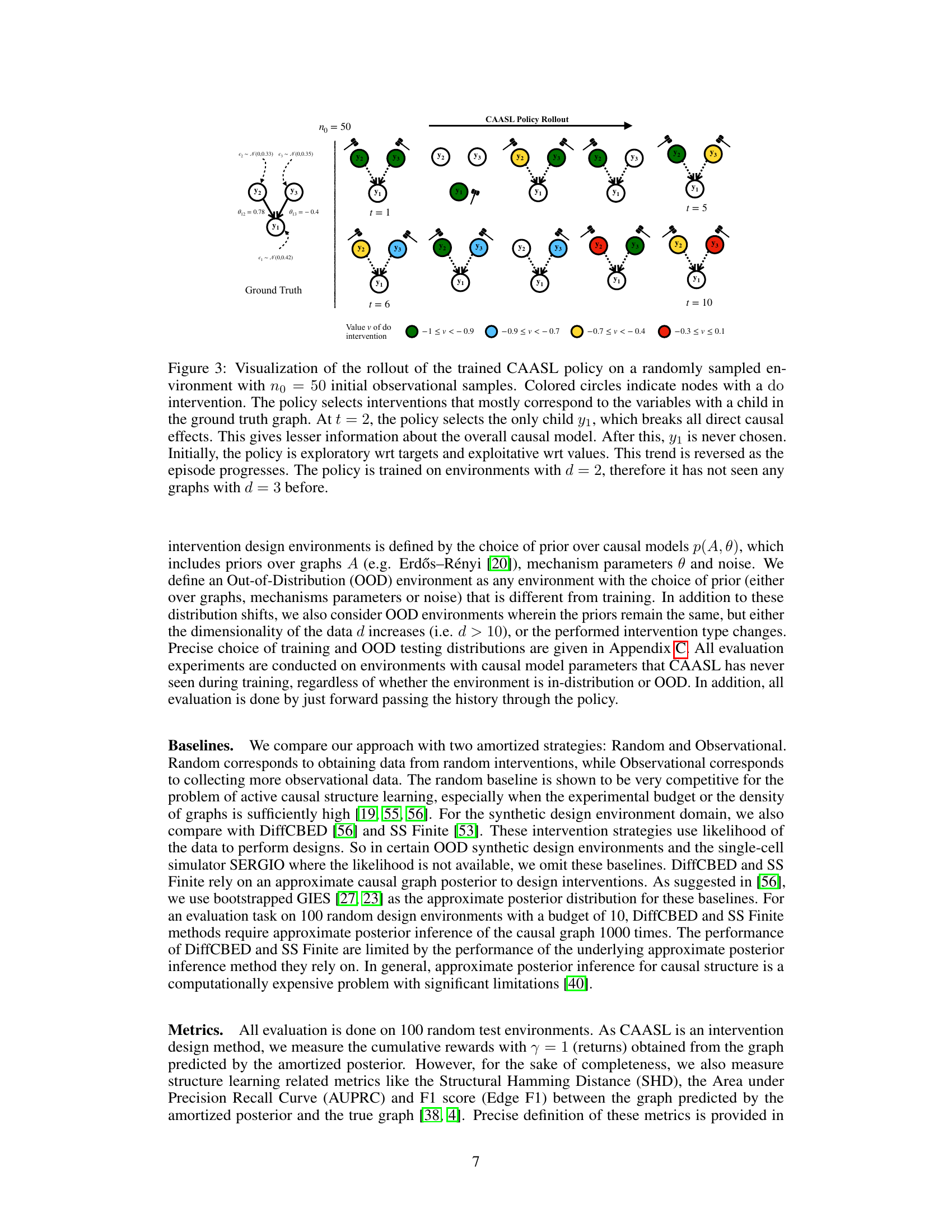
🔼 This figure presents the performance comparison of different intervention strategies, including CAASL, Random, Observational, DiffCBED, and SS Finite, in terms of returns, SHD, AUPRC, and Edge F1 over 10 intervention iterations. The results show that CAASL consistently outperforms the baselines across all metrics. The shaded area in each plot represents the 95% confidence interval, indicating the variability of the results.
read the caption
Figure 4: Amortization results of various intervention strategies on 100 random test environments. CAASL significantly outperforms other intervention strategies. Shaded area represents 95% CI.

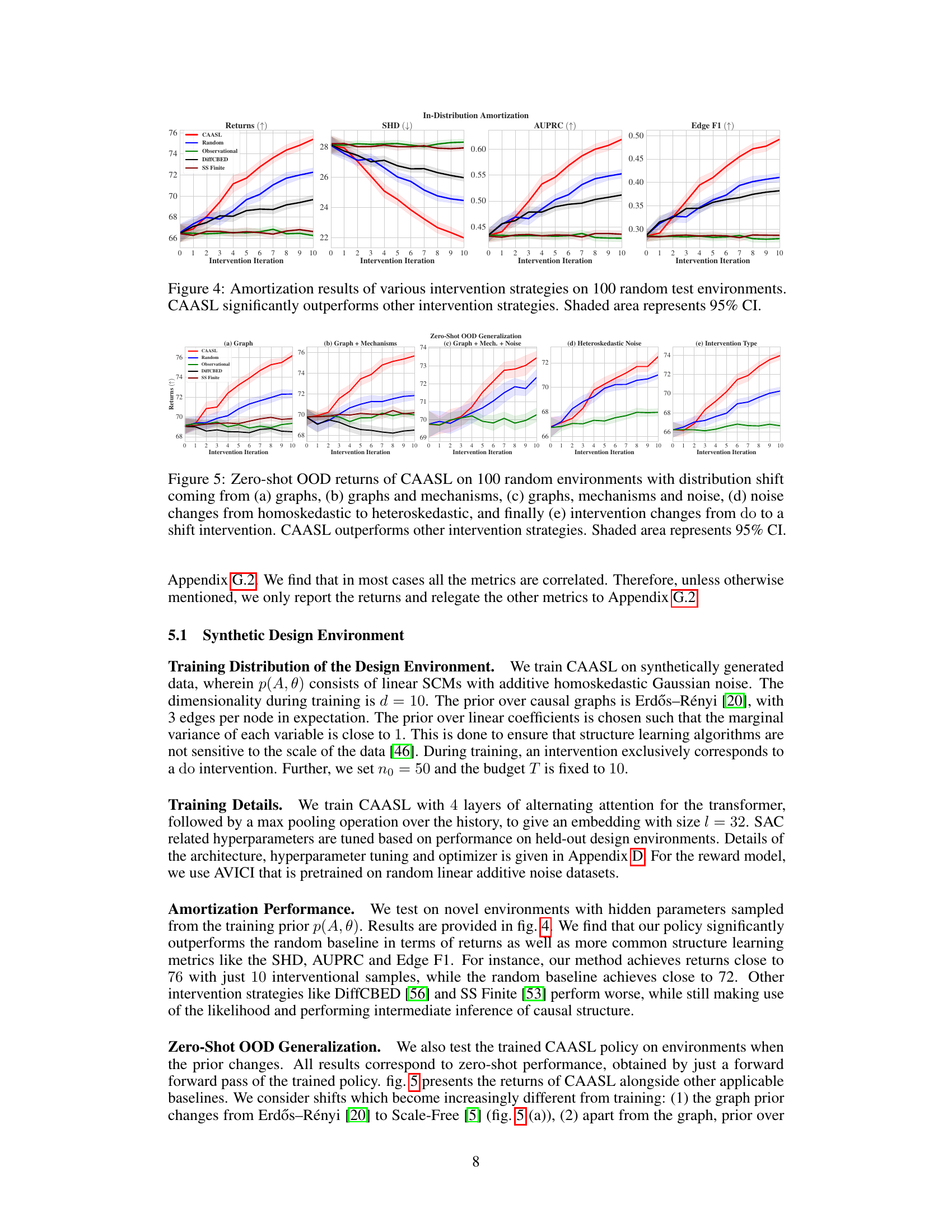
🔼 This figure shows the zero-shot out-of-distribution (OOD) generalization performance of the Causal Amortized Active Structure Learning (CAASL) method across five different OOD scenarios. Each subfigure represents a different type of distribution shift from the training data: (a) changes in the graph structure (prior over graphs), (b) changes in both graph structure and mechanisms (prior over parameters), (c) changes in graph structure, mechanisms, and noise distribution, (d) switching from homoskedastic noise to heteroskedastic noise, and (e) changing the intervention type from a perfect intervention to a shift intervention. The CAASL method consistently outperforms other strategies (Random, Observational, DiffCBED, SS Finite) in all scenarios, demonstrating its robustness to distribution shifts. The shaded area in each plot represents the 95% confidence interval.
read the caption
Figure 5: Zero-shot OOD returns of CAASL on 100 random environments with distribution shift coming from (a) graphs, (b) graphs and mechanisms, (c) graphs, mechanisms and noise, (d) noise changes from homoskedastic to heteroskedastic, and finally (e) intervention changes from do to a shift intervention. CAASL outperforms other intervention strategies. Shaded area represents 95% CI.
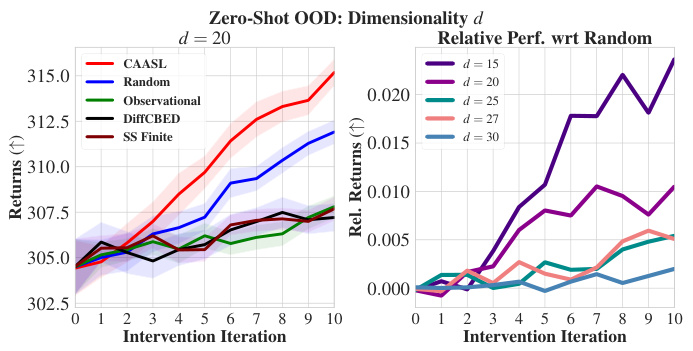
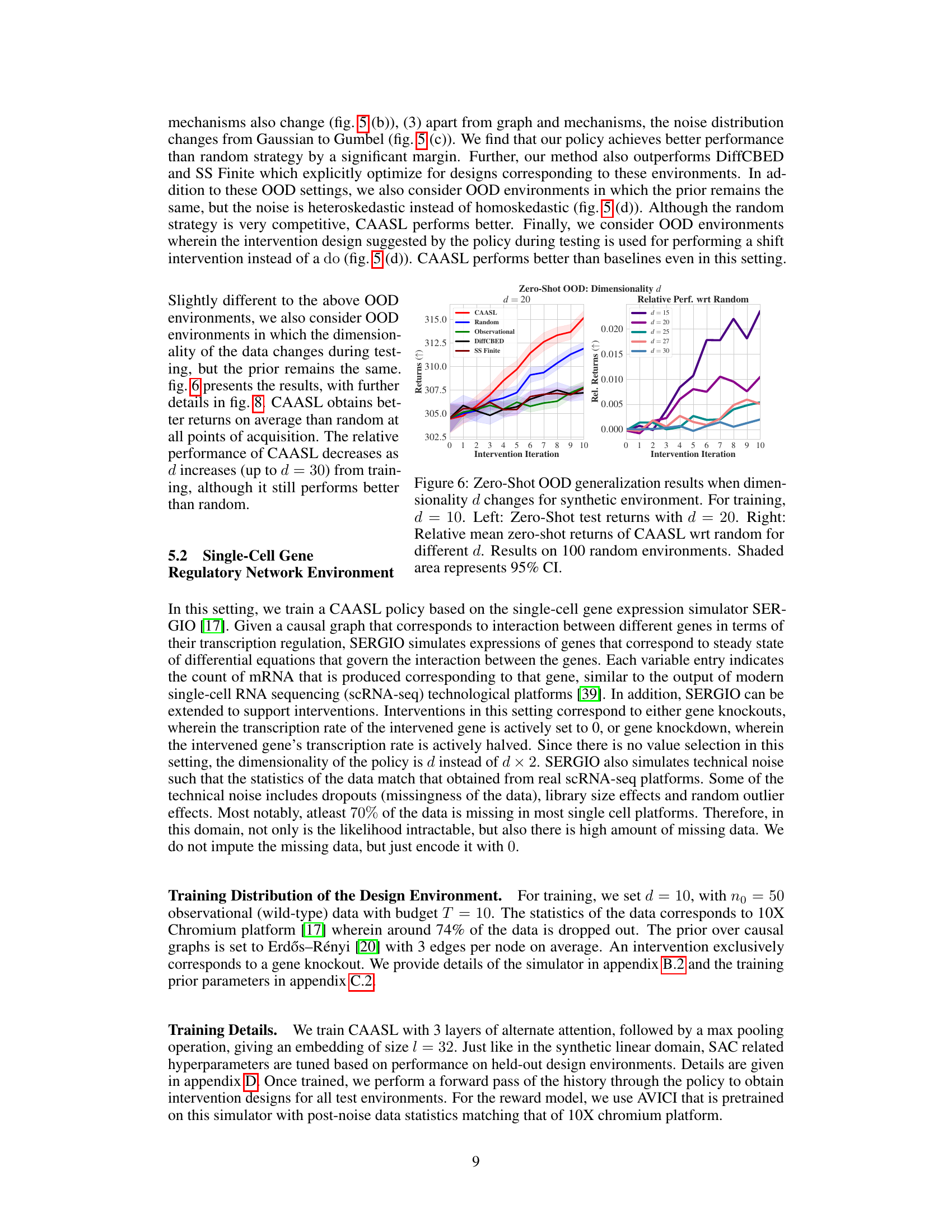
🔼 This figure demonstrates the zero-shot out-of-distribution generalization performance of CAASL when the dimensionality of the data increases during testing. The left panel displays the test returns for a dimensionality of d=20, showing the significant improvement of CAASL over baselines. The right panel shows the relative performance of CAASL with respect to a random baseline for various dimensionalities (d=15, 20, 25, 27, 30), highlighting the robustness of CAASL even when the dimensionality increases during the testing phase.
read the caption
Figure 6: Zero-Shot OOD generalization results when dimensionality d changes for synthetic environment. For training, d = 10. Left: Zero-Shot test returns with d = 20. Right: Relative mean zero-shot returns of CAASL wrt random for different d. Results on 100 random environments. Shaded area represents 95% CI.

🔼 This figure displays the performance of CAASL and baselines in the SERGIO environment under various conditions. Panel (a) shows in-distribution results, where the model is tested on data similar to that used for training. Panels (b) through (e) demonstrate the zero-shot out-of-distribution generalization capabilities of the method, showing its performance when the underlying generative model changes (different graphs, noise characteristics, intervention types, noisy interventions). Each panel shows the cumulative reward obtained over 10 intervention steps, highlighting the resilience of CAASL in various challenging scenarios. Shaded areas represent the 95% confidence interval.
read the caption
Figure 7: Results on SERGIO environment with 100 random environments. (a) corresponds to in-distribution performance, (b)-(e) correspond to zero-shot OOD performance with distribution shift coming from either (b) graphs, (c) technical noise, (d) intervention changing to a gene-knockdown (e) Noisy interventions, which include off-target effects. Shaded area represents 95% CI.

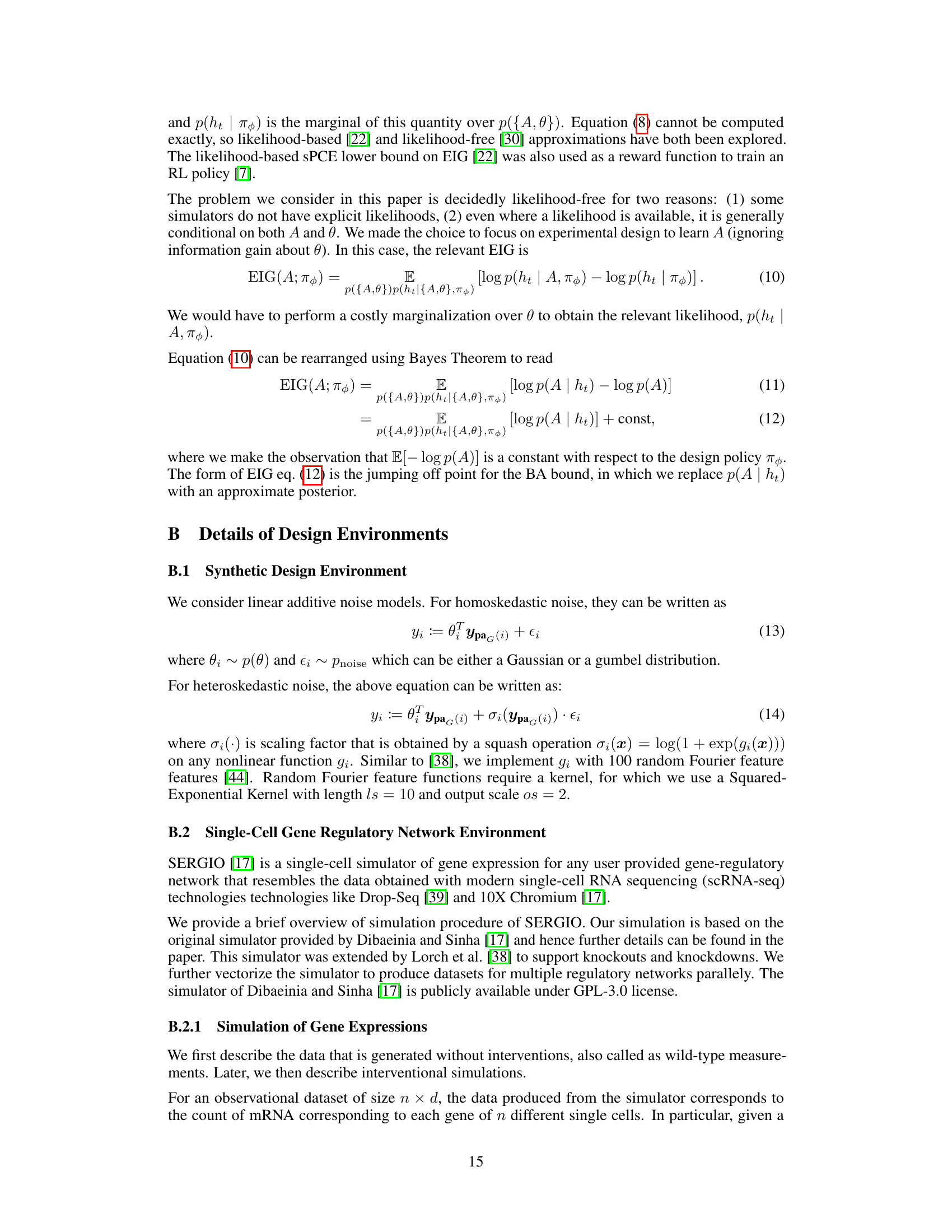
🔼 This figure shows the results of a zero-shot out-of-distribution (OOD) generalization experiment, where the dimensionality of the data increases. The experiment was performed on a synthetic dataset, and the results show the returns (cumulative rewards) over 10 intervention iterations. Four different dimensionalities (d = 15, 20, 25, 30) are tested, and the performance of CAASL is compared against two baseline methods: random interventions and purely observational data. The shaded areas represent the 95% confidence intervals, indicating the uncertainty in the results. CAASL consistently outperforms the baselines, demonstrating its ability to generalize to higher-dimensional data unseen during training.
read the caption
Figure 8: Results of zero-shot OOD generalization when dimensionality of the data increases in the synthetic environment. Results are performed on 100 random test environments. Shaded area represents 95% CI.
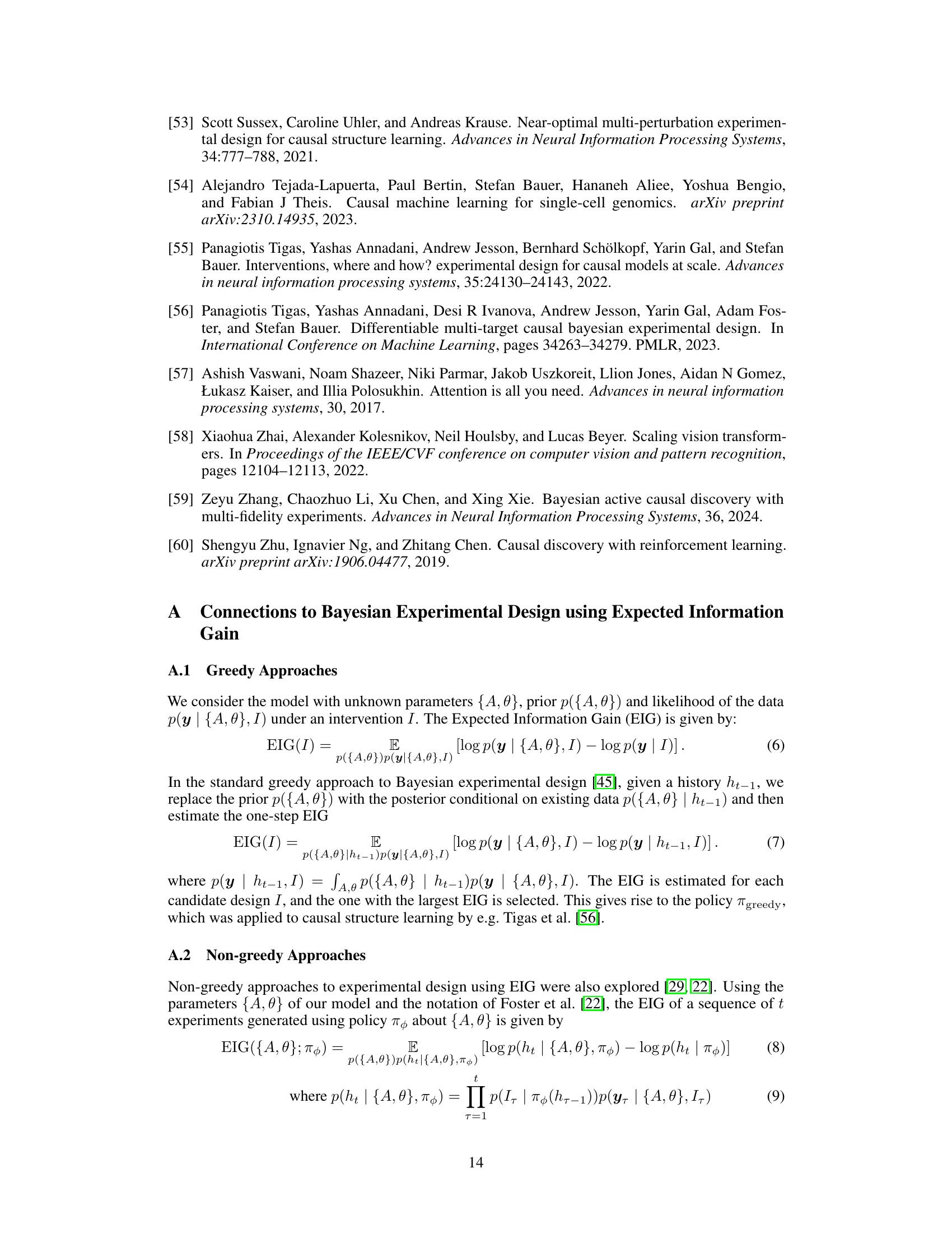
🔼 This figure displays the results of a zero-shot out-of-distribution (OOD) generalization experiment where the dimensionality (d) of the synthetic design environment is varied. The training data used d=10, while the test data used d=15, 20, 25, 27, and 30. The left panel shows the zero-shot test returns for d=20, illustrating the performance of CAASL, random, and observational strategies. The right panel shows the relative mean returns of CAASL compared to the random strategy for different values of d, highlighting how the relative performance changes as dimensionality increases. Shaded areas indicate 95% confidence intervals.
read the caption
Figure 6: Zero-Shot OOD generalization results when dimensionality d changes for synthetic environment. For training, d = 10. Left: Zero-Shot test returns with d = 20. Right: Relative mean zero-shot returns of CAASL wrt random for different d. Results on 100 random environments. Shaded area represents 95% CI.

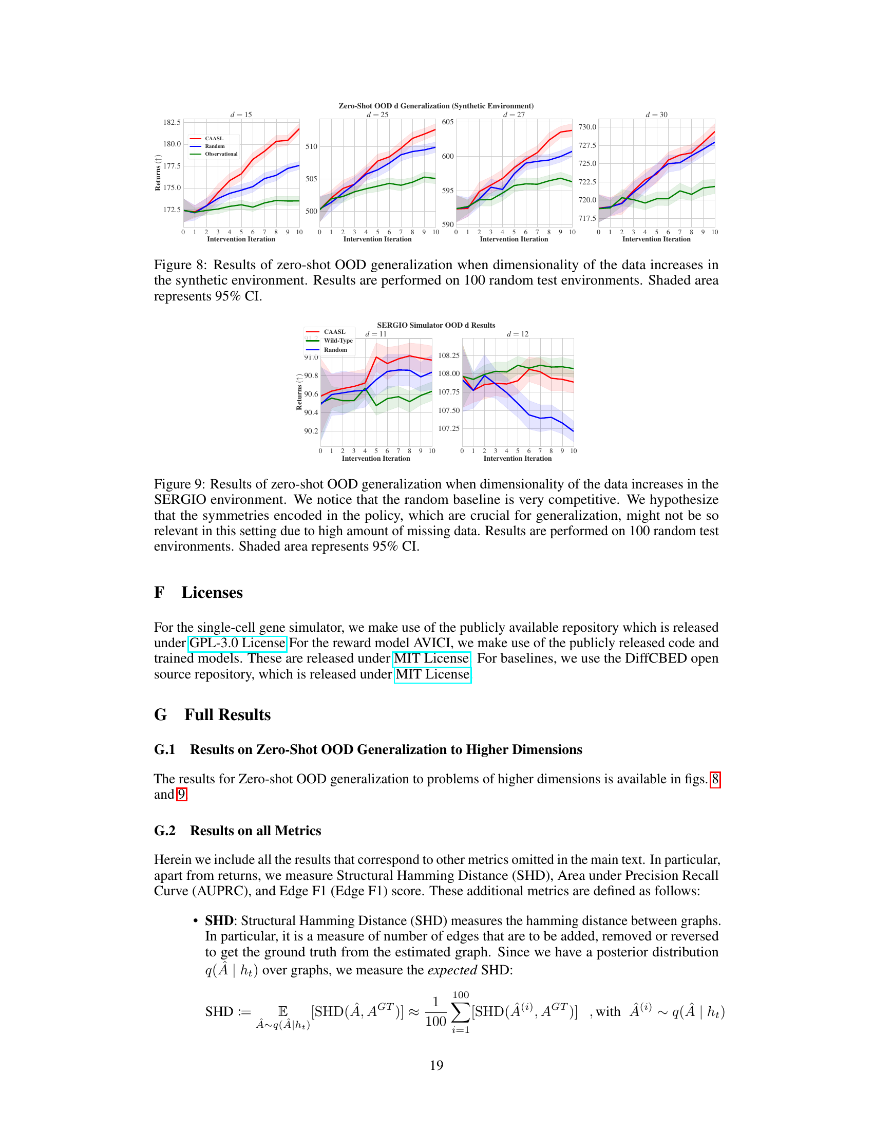
🔼 This figure presents the performance comparison of different intervention strategies, including CAASL, Random, and Observational methods, over 100 random test environments. The results are displayed for 10 intervention iterations, showing the return values obtained. CAASL demonstrates significantly better performance than other strategies, as indicated by the higher return values. The shaded areas represent the 95% confidence intervals, illustrating the statistical significance of the results.
read the caption
Figure 4: Amortization results of various intervention strategies on 100 random test environments. CAASL significantly outperforms other intervention strategies. Shaded area represents 95% CI.

🔼 The figure shows the performance of different intervention strategies on 100 random test environments over 10 intervention iterations. The y-axis represents the cumulative rewards, SHD, AUPRC, and Edge F1 score. CAASL consistently outperforms other methods (Random, Observational, DiffCBED, and SS Finite) across all metrics, demonstrating its effectiveness in sample-efficient causal structure learning. The shaded areas represent the 95% confidence intervals.
read the caption
Figure 4: Amortization results of various intervention strategies on 100 random test environments. CAASL significantly outperforms other intervention strategies. Shaded area represents 95% CI.

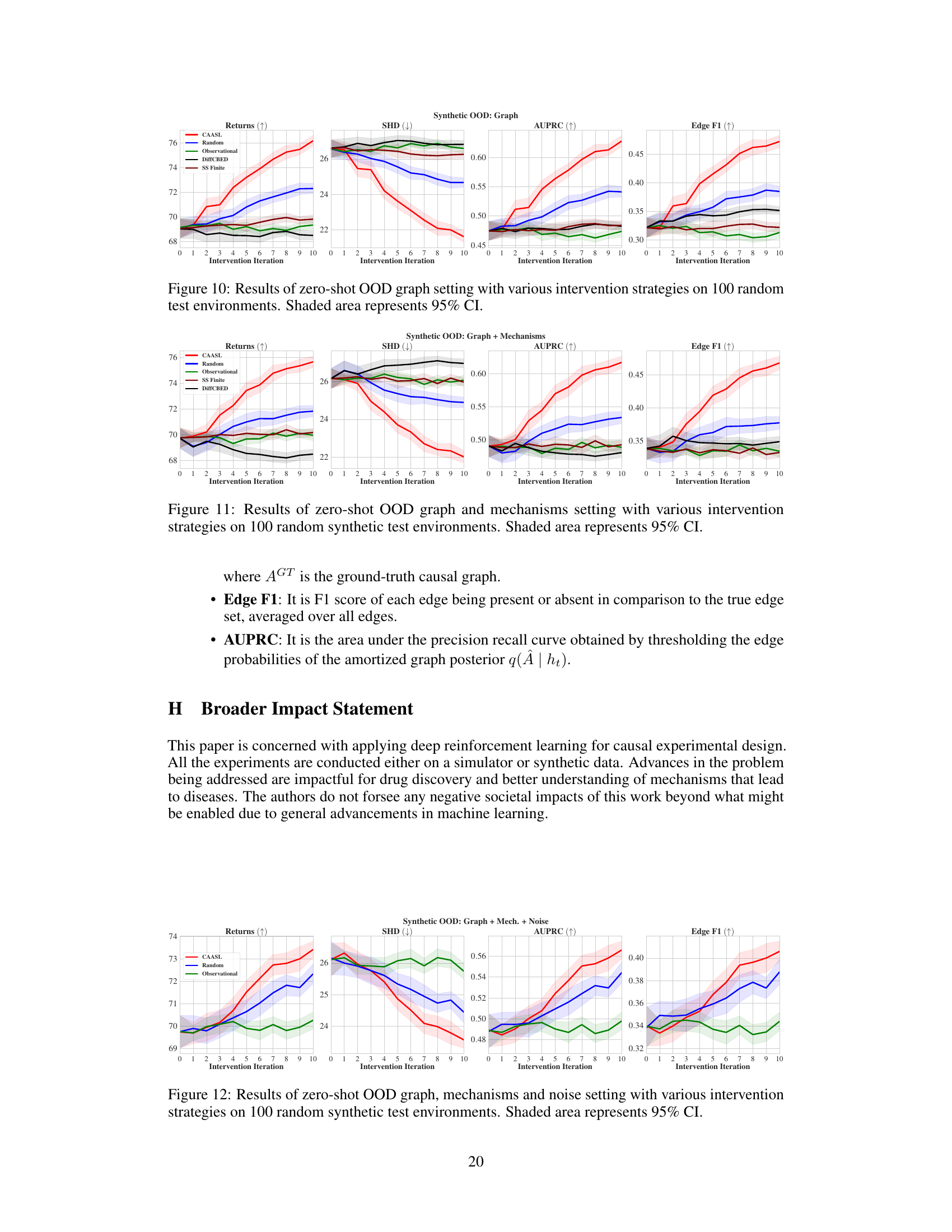
🔼 The figure displays the performance of various intervention strategies in a zero-shot out-of-distribution (OOD) setting where the data generation process deviates from the training data in terms of graph structure, mechanisms, and noise. The plot includes the returns (cumulative reward), Structural Hamming Distance (SHD), Area Under the Precision-Recall Curve (AUPRC), and Edge F1-score. CAASL significantly outperforms the baseline strategies (Random and Observational) across all metrics. The shaded regions indicate the 95% confidence intervals, highlighting the statistical significance of the results.
read the caption
Figure 12: Results of zero-shot OOD graph, mechanisms and noise setting with various intervention strategies on 100 random synthetic test environments. Shaded area represents 95% CI.

🔼 This figure presents the performance comparison of different intervention strategies, including CAASL, Random, and Observational, across 10 returns, SHD, AUPRC, and Edge F1 metrics. The results are obtained from 100 random test environments. CAASL consistently outperforms the other methods, showcasing its effectiveness in active intervention design for causal structure learning. The shaded areas indicate the 95% confidence intervals.
read the caption
Figure 4: Amortization results of various intervention strategies on 100 random test environments. CAASL significantly outperforms other intervention strategies. Shaded area represents 95% CI.

🔼 This figure presents the comparison of different intervention strategies on 100 random test environments. The y-axis shows the performance metrics (Returns, SHD, AUPRC, Edge F1), and the x-axis represents intervention iterations. The lines represent CAASL, Random, and Observational intervention strategies. CAASL consistently outperforms the others, indicating the effectiveness of the proposed method in learning causal structure from data acquired through its adaptive intervention design.
read the caption
Figure 4: Amortization results of various intervention strategies on 100 random test environments. CAASL significantly outperforms other intervention strategies. Shaded area represents 95% CI.

🔼 This figure shows the performance of different intervention strategies over 10 iterations on 100 random test environments. The x-axis represents the intervention iteration, and the y-axis shows the performance metric (returns, SHD, AUPRC, Edge F1). CAASL consistently outperforms both Random and Observational strategies across all metrics, indicating its superior ability to design informative interventions for causal structure learning. The shaded areas represent 95% confidence intervals, highlighting the statistical significance of the results.
read the caption
Figure 4: Amortization results of various intervention strategies on 100 random test environments. CAASL significantly outperforms other intervention strategies. Shaded area represents 95% CI.

🔼 The figure shows the performance of different intervention strategies, including CAASL (Causal Amortized Active Structure Learning), Random, and Observational, across 10 intervention iterations on 100 random test environments. CAASL consistently outperforms the other methods, demonstrating its effectiveness in efficiently acquiring data for causal structure learning. The shaded areas indicate the 95% confidence intervals.
read the caption
Figure 4: Amortization results of various intervention strategies on 100 random test environments. CAASL significantly outperforms other intervention strategies. Shaded area represents 95% CI.

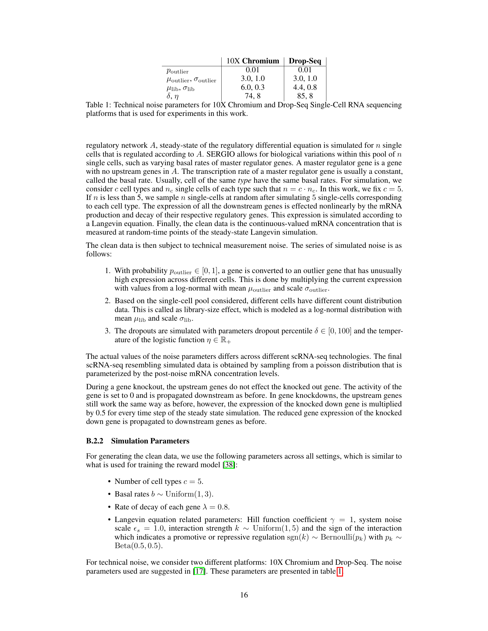
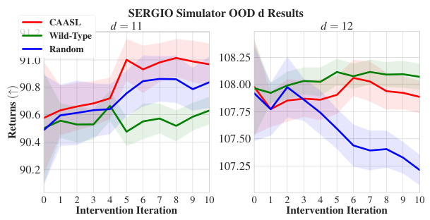
🔼 This figure shows the results of the CAASL policy and baselines (Wild-type and Random) on the SERGIO environment for in-distribution and various out-of-distribution (OOD) settings. The in-distribution setting evaluates the amortization capability of the policy on the training distribution. The OOD settings evaluate the generalization ability of the policy to new environments with distribution shifts in terms of graph structure, technical noise (scRNA-seq platform), intervention type, and noisy interventions (off-target effects). The shaded area represents the 95% confidence interval for each metric across 100 random environments.
read the caption
Figure 7: Results on SERGIO environment with 100 random environments. (a) corresponds to in-distribution performance, (b)-(e) correspond to zero-shot OOD performance with distribution shift coming from either (b) graphs, (c) technical noise, (d) intervention changing to a gene-knockdown (e) Noisy interventions, which include off-target effects. Shaded area represents 95% CI.

🔼 This figure displays the performance of CAASL and other intervention strategies (Random and Observational) over 10 interventions on 100 different synthetic test environments. The y-axis shows the cumulative reward, and the x-axis represents the intervention iteration. CAASL consistently demonstrates superior performance compared to Random and Observational approaches, as indicated by the significantly higher cumulative rewards. The shaded regions represent the 95% confidence intervals for each strategy.
read the caption
Figure 4: Amortization results of various intervention strategies on 100 random test environments. CAASL significantly outperforms other intervention strategies. Shaded area represents 95% CI.

🔼 This figure shows the results of a zero-shot out-of-distribution (OOD) generalization experiment. In the experiment, noisy interventions (10% probability of off-target effects or failed interventions) were introduced into the SERGIO gene regulatory network simulator. The figure displays four metrics across 10 intervention iterations: Returns (cumulative reward), SHD (Structural Hamming Distance, lower is better), AUPRC (Area Under the Precision-Recall Curve, higher is better), and Edge F1 (F1 score for edge accuracy, higher is better). The results are compared across three intervention strategies: CAASL (the proposed method), Wild-Type (observational data), and Random (random interventions). Shaded areas represent 95% confidence intervals. The results demonstrate CAASL’s robustness in handling noisy interventions, outperforming both the Wild-Type and Random strategies.
read the caption
Figure 19: Results of zero-shot OOD noisy gene knockouts with various intervention strategies on 100 random SERGIO test environments. Shaded area represents 95% CI.
Full paper#

