TL;DR#
Partial Information Decomposition (PID) is a valuable tool for understanding complex systems but its computation is challenging, especially for continuous distributions. Existing methods often rely on numerical approximations, which can be computationally expensive and lack accuracy. This necessitates the development of efficient and accurate analytical solutions.
This research tackles this challenge head-on. The authors present analytical PID calculations for various distributions, including those commonly used in neuroscience. Their approach leverages a novel link between PID and the fields of data thinning and fission, enabling the derivation of analytical results for a broader class of distributions. They further enhance the practical applicability of PID by providing an analytical upper bound for approximating PID computations, confirmed to be remarkably precise through rigorous simulation testing.
Key Takeaways#
Why does it matter?#
This paper is crucial because it significantly advances the analytical computation of Partial Information Decomposition (PID), a challenging problem in various fields. By providing analytical solutions for a wide range of distributions, it offers more accurate and efficient PID calculations, enabling deeper insights into complex systems. The theoretical links established between PID and data thinning/fission open new avenues for research and development of advanced analytical tools.
Visual Insights#

🔼 The figure shows the results of a simulation comparing the analytical approximation of the mutual information (QA) to the numerical approximation (QN) for 20 different function pairs and 75 different prior distributions for M. The box plots in (a) and (b) illustrate the differences between QA and QN mutual information values, and the numerical estimates respectively. Plot (c) shows the percentage difference between the median of QA and QN for each of the 20 pairs.
read the caption
Figure 1: a and b, respectively, show the box plot of the difference IQA(M, X, Y) – IQN(M, X, Y) and the corresponding values of IQN(M, X, Y) for the 20 different function pairs across the 75 different P(M) distributions. The light-blue dots show the corresponding data points used for making the box plots. c shows the ratio of the median difference IQA(M, X, Y) – IQN(M, X, Y) and the median value of IQN(M, X, Y) in percentage, for each function pair.
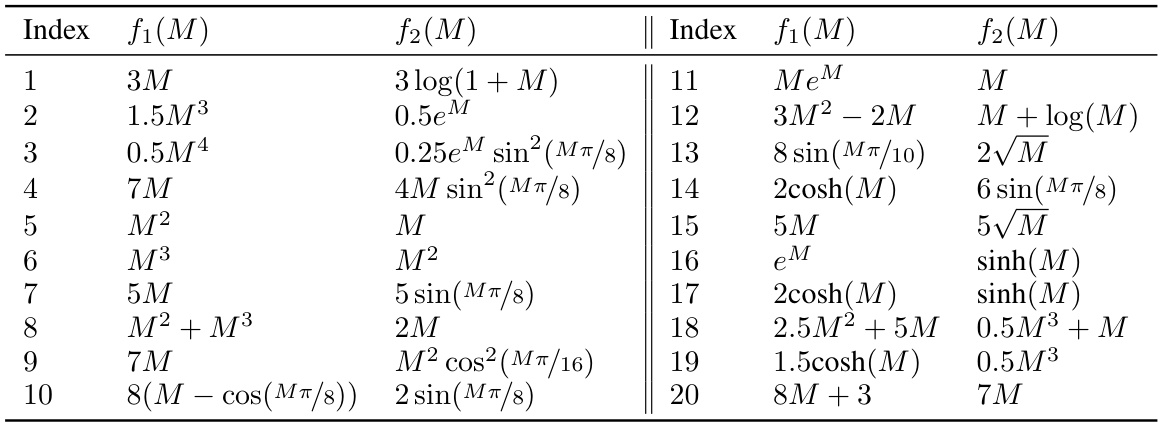
🔼 This table lists 20 pairs of functions f1(M) and f2(M) used in a simulation study to compare analytical and numerical estimations of mutual information. The simulation uses Poisson distributions, and the table indexes the function pairs used in the study, shown graphically in Figure 1.
read the caption
Table 1: Table 1 lists the 20 different function pairs used in the simulation study described in Sec. 6 for comparing the analytical estimate of the minimizing distribution of (2) proposed in Sec. 6 with the corresponding ground-truth numerical estimate. The index in Table 1 maps the corresponding function pair to the results shown in Fig. 1. To illustrate, the number 1 on the x-axis of all the plots shown in Fig. 1 corresponds to the function pair with index 1 in Table 1.
In-depth insights#
PID’s Analytical Advance#
The research paper section titled “PID’s Analytical Advance” would likely detail the significant breakthrough of deriving analytical solutions for Partial Information Decomposition (PID) calculations. This is a major contribution because computing PID numerically is often computationally expensive and can be prone to approximation errors. The analytical advances likely center around identifying specific families of probability distributions (e.g., stable distributions, convolution-closed distributions) where closed-form PID solutions exist. The core innovation probably involves a clever mathematical manipulation or a novel theoretical framework to simplify the complex optimization problem inherent in PID calculation. This simplification might leverage inherent properties of the chosen distribution families, such as their behavior under convolution or affine transformations, to directly obtain the unique, redundant, and synergistic information components. The section would then present these analytical solutions, potentially accompanied by detailed proofs and illustrative examples to showcase their application and practical utility. The results likely highlight the benefit of these analytical expressions in reducing computational cost, increasing accuracy, and providing deeper theoretical insight into information interactions within complex systems. Overall, this section would demonstrate a notable advancement in PID’s applicability, expanding its use beyond numerical approximations to more readily analytical calculation, paving the way for wider adoption and more profound application in various fields.
Stable Dist. PID#
The section on Stable Distribution PID likely explores extending the analytical calculation of Partial Information Decomposition (PID) beyond the Gaussian case, a significant limitation of previous work. The authors probably leverage the properties of stable distributions, which include Gaussian distributions as a special case, to derive analytical expressions for PID components. This generalization is crucial as it allows the application of PID to broader scenarios in fields like neuroscience, where data often displays heavy tails and non-Gaussian characteristics. The core argument likely involves demonstrating that a specific form of affine dependence between the source and target variables, coupled with the use of stable distributions, guarantees that at least one unique information term in the PID vanishes, simplifying the computation of the remaining terms. Analytical expressions derived for several well-known stable distributions (e.g., Poisson, Cauchy, Lévy) would showcase the practical value and extendability of the approach. The results likely demonstrate the theoretical link between PID and data thinning/fission, highlighting its usefulness in information-theoretic analysis. However, potential limitations might arise from the assumptions of affine dependence and the inherent difficulty of dealing with the general form of stable distributions analytically.
Data Thinning & PID#
The connection between data thinning and partial information decomposition (PID) presents a novel and insightful approach to analytically compute PID. Data thinning, a technique for splitting random variables, offers a pathway to constructing Markov chains that simplify PID calculations. By strategically decomposing a source variable into components that match the other sources’ distributions, redundant and unique information terms can be directly determined, effectively bypassing the computationally intensive optimization problems usually associated with PID estimation. This theoretical link facilitates the analytical calculation of PID for diverse systems, extending the applicability beyond the previously limited Gaussian case. The key advantage lies in converting a complex optimization problem into an easier analytical derivation. However, the reliance on specific distribution properties (like convolution-closure) limits the generalizability of this method. Future work should focus on expanding this approach to broader distribution classes and exploring its limitations to build a more robust framework for PID computation.
Convolution-Closed PID#
The concept of “Convolution-Closed PID” suggests an intriguing line of inquiry within the field of Partial Information Decomposition (PID). It implies leveraging the mathematical properties of convolution-closed distributions to derive analytical solutions for PID, avoiding computationally intensive numerical methods. This approach promises significant advancements, potentially broadening PID’s applicability to a wider range of systems and datasets. The core idea is that the sum of independent random variables from a convolution-closed family remains within the same family, simplifying the often complex optimization problems involved in PID calculations. By identifying specific convolution-closed distributions relevant to particular applications, such as neuroscience, researchers could potentially unlock new analytical insights into information processing mechanisms. However, exploring “Convolution-Closed PID” would also necessitate a thorough investigation into the limitations of this approach, examining whether this technique can be successfully generalized beyond specific distribution families and considering potential tradeoffs between analytical tractability and the generality of results. The tightness and limitations of any analytical bounds derived using this method should also be thoroughly examined.
PID Future Works#
The ‘PID Future Works’ section of a research paper would ideally delve into promising avenues for extending partial information decomposition (PID) research. This would likely involve extending PID to more complex systems, moving beyond the bivariate case explored in many current works. The paper might suggest investigating high-dimensional data or incorporate time-series analysis to handle dynamic systems more effectively. Another key area is developing more robust and efficient computational methods for PID calculations, especially for continuous distributions where numerical approximations are often necessary. Further exploration of the relationship between PID and other information-theoretic frameworks could yield valuable insights. Finally, applying PID to new application domains is crucial; the authors could highlight areas like machine learning, causal inference, and complex systems where PID’s ability to disentangle information sources could significantly improve our understanding. Addressing the challenges in these areas would solidify PID’s status as a powerful analytical tool and open up exciting possibilities for future investigation.
More visual insights#
More on figures
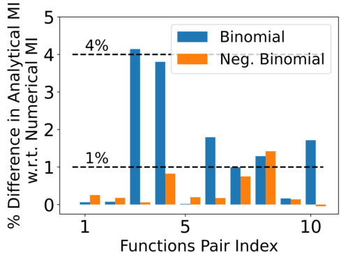
🔼 This figure shows the results of a simulation study to evaluate the tightness of an analytical upper bound for approximating the solution of the constrained minimization problem involved in computing the Partial Information Decomposition (PID) terms. The study considers 20 different pairs of functions and 75 different prior distributions. The plots compare the analytical estimate with numerical ground truth estimates for each function pair, showing the difference in mutual information (MI) and the percentage difference in MI, with the light blue dots indicating individual data points.
read the caption
Figure 1: a and b, respectively, show the box plot of the difference IQA(M, X, Y) – IQN(M, X, Y) and the corresponding values of IQN(M, X, Y) for the 20 different function pairs across the 75 different P(M) distributions. The light-blue dots show the corresponding data points used for making the box plots. c shows the ratio of the median difference IQA(M, X, Y) – IQN(M, X, Y) and the median value of IQN(M, X, Y) in percentage, for each function pair.
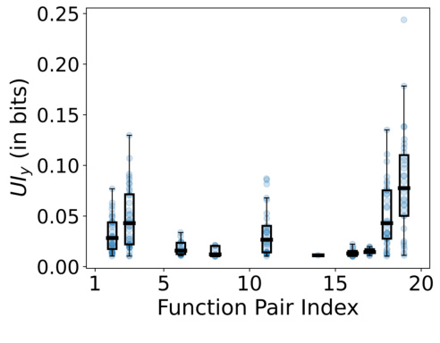
🔼 This figure compares the analytical estimate of the upper bound with the ground truth numerical estimate. The upper bound is derived using the assumptions in (9), and its performance is evaluated for 20 different function pairs and 75 different distributions of P(M). The plots shown in the figure illustrate the differences in the analytical and numerical estimates, the values of the numerical estimates, and their ratio in percentage for each function pair. It shows the accuracy and goodness of the analytical upper bound for solving the minimization problem.
read the caption
Figure 1: a and b, respectively, show the box plot of the difference IQA(M, X, Y) – IQN(M, X, Y) and the corresponding values of IQN(M, X, Y) for the 20 different function pairs across the 75 different P(M) distributions. The light-blue dots show the corresponding data points used for making the box plots. c shows the ratio of the median difference IQA(M, X, Y) – IQN(M, X, Y) and the median value of IQN(M, X, Y) in percentage, for each function pair.
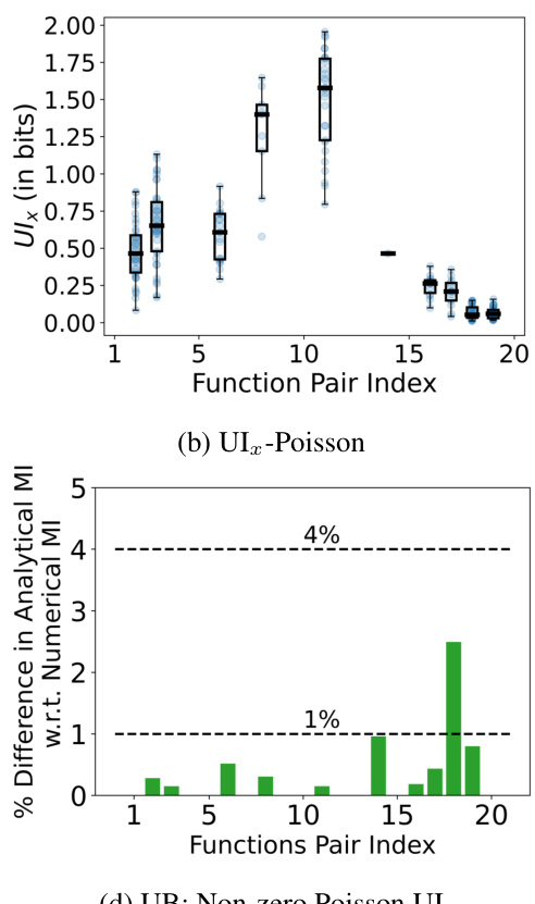
🔼 The figure shows the results of a simulation study to evaluate the tightness of the analytical upper bound derived in Section 6. Subfigure (a) and (b) present box plots comparing the analytical mutual information (IQA) against the numerical mutual information (IQN) for 20 different function pairs across 75 different prior distributions P(M). The difference between IQA and IQN, and IQN are plotted separately. The third subfigure (c) shows the percentage difference between the median of IQA and IQN compared to the median of IQN for the same function pairs, highlighting the tightness of the approximation.
read the caption
Figure 1: a and b, respectively, show the box plot of the difference IQA(M, X, Y) – IQN(M, X, Y) and the corresponding values of IQN(M, X, Y) for the 20 different function pairs across the 75 different P(M) distributions. The light-blue dots show the corresponding data points used for making the box plots. c shows the ratio of the median difference IQA(M, X, Y) – IQN(M, X, Y) and the median value of IQN(M, X, Y) in percentage, for each function pair.
Full paper#
