TL;DR#
Machine learning heavily relies on loss functions to quantify the difference between model predictions and actual values. Existing Fenchel-Young losses, while widely used, present room for improvement. They are implicitly associated with a specific prediction mapping or ‘link function.’
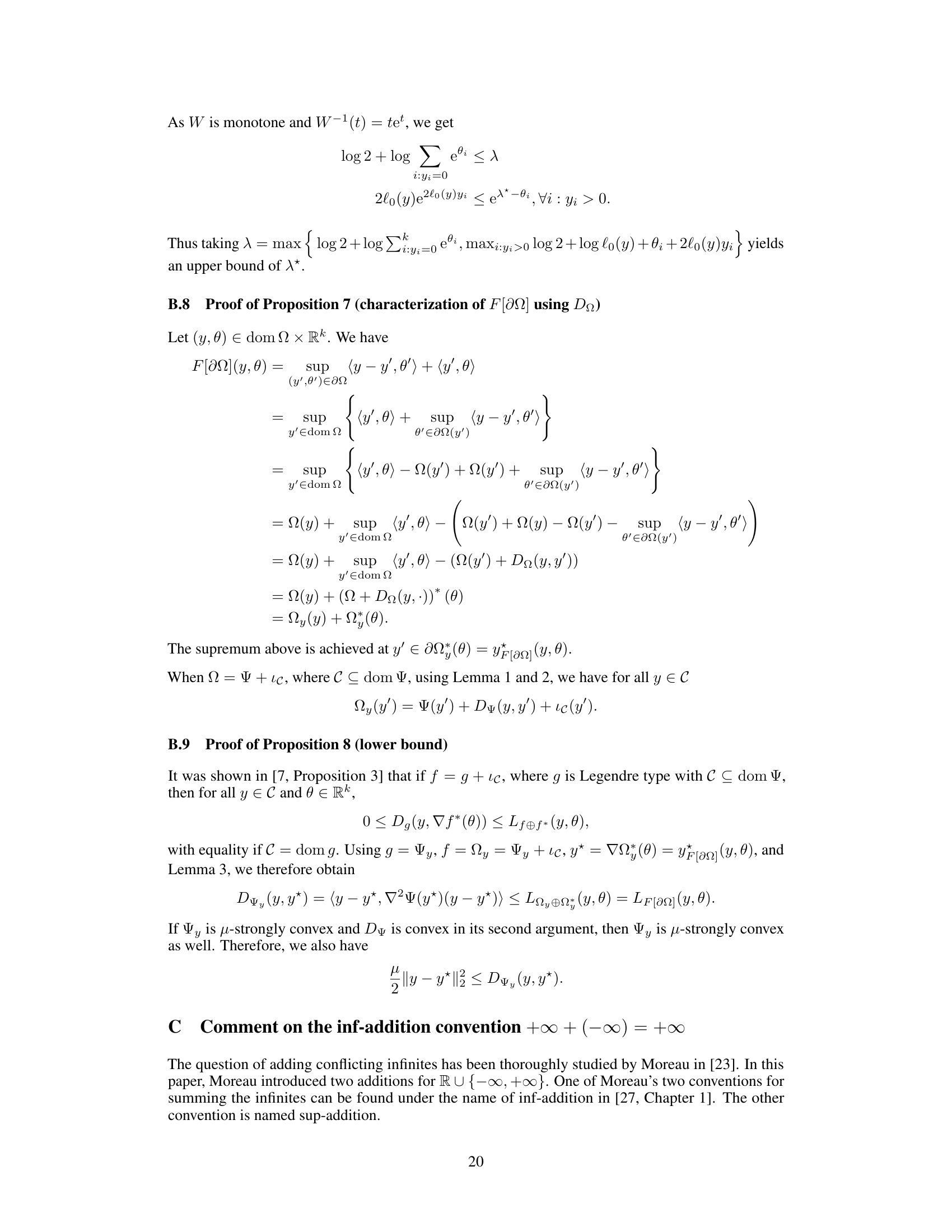
This paper introduces Fitzpatrick losses, a novel family of loss functions. These losses leverage the Fitzpatrick function from maximal monotone operator theory to achieve a refined Fenchel-Young inequality resulting in tighter bounds. The new losses retain the same link function as Fenchel-Young losses which is crucial for prediction consistency. Empirical studies on various datasets demonstrate that these tighter losses yield superior performance for probability classification, particularly in label proportion estimation.
Key Takeaways#
Why does it matter?#
This paper is important because it introduces Fitzpatrick losses, a new family of loss functions that are tighter than existing Fenchel-Young losses while maintaining the same link function. This offers improved accuracy and efficiency in machine learning tasks, opening new avenues for research in loss function design and optimization. The findings are relevant to current trends in developing more efficient and accurate machine learning models.
Visual Insights#
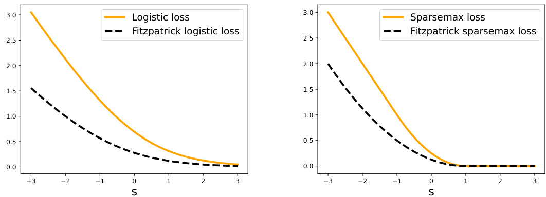
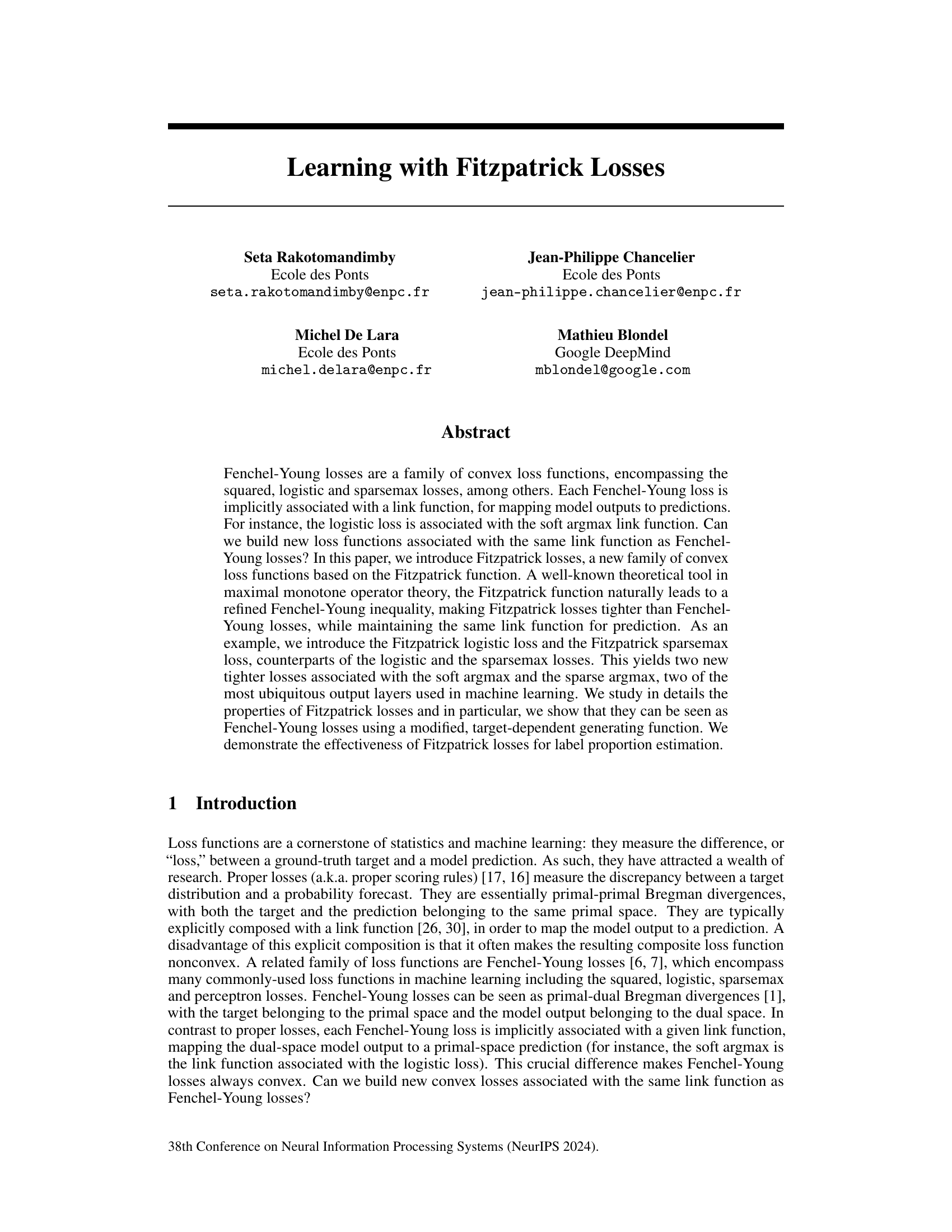
🔼 The figure shows a comparison of the logistic loss and the Fitzpatrick logistic loss, and also the sparsemax loss and the Fitzpatrick sparsemax loss. It demonstrates that the Fitzpatrick losses provide tighter lower bounds than their corresponding Fenchel-Young counterparts while using the same link functions. The plots visualize the loss values, L(y, θ), for varying values of s, where y is a one-hot encoded vector and θ is a vector with s as its first element and 0 for the remaining elements. This shows the improved tightness of Fitzpatrick losses.
read the caption
Figure 1: We introduce Fitzpatrick losses, a new family of loss functions generated by a convex regularization function Ω, that lower-bound Fenchel-Young losses generated by the same Ω, while maintaining the same link function ŷn = ΠΩ*. In particular, we use our framework to instantiate the counterparts of the logistic and sparsemax losses, two instances of Fenchel-Young losses, associated with the soft argmax and the sparse argmax. In the figures above, we plot L(y, 0), where y = e1, 0 = (s, 0) and L ∈ {LF[an], Lo⊕n* }, confirming the lower-bound property.

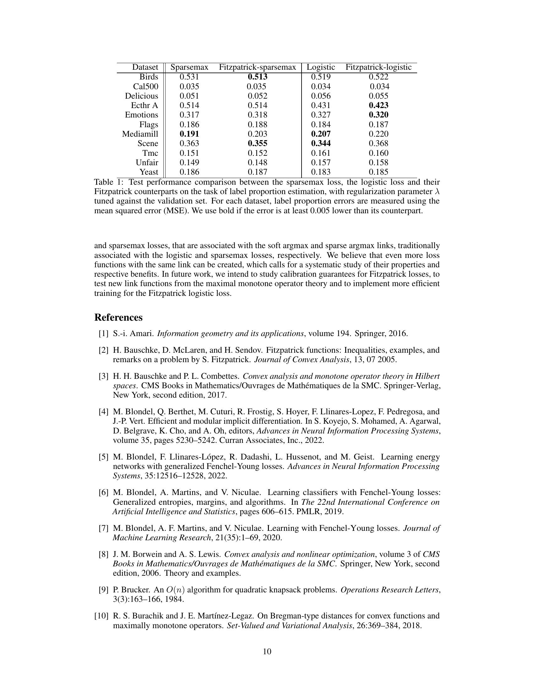
🔼 This table compares the performance of four different loss functions (sparsemax, Fitzpatrick sparsemax, logistic, and Fitzpatrick logistic) on eleven different datasets. The performance metric is mean squared error (MSE), which measures the difference between predicted and actual label proportions. Bold values indicate cases where the MSE is at least 0.005 lower than the corresponding non-Fitzpatrick loss.
read the caption
Table 1: Test performance comparison between the sparsemax loss, the logistic loss and their Fitzpatrick counterparts on the task of label proportion estimation, with regularization parameter λ tuned against the validation set. For each dataset, label proportion errors are measured using the mean squared error (MSE). We use bold if the error is at least 0.005 lower than its counterpart.
In-depth insights#
Fitzpatrick Losses#
The concept of “Fitzpatrick Losses” introduces a novel family of convex loss functions in machine learning, offering tighter bounds than traditional Fenchel-Young losses while maintaining the same link function for predictions. This tighter bound is achieved through the utilization of the Fitzpatrick function, a theoretical tool from maximal monotone operator theory. The paper presents the Fitzpatrick logistic and sparsemax losses as specific instances, demonstrating their effectiveness in probabilistic classification tasks. A key advantage is the preservation of the same link function (e.g., softmax for logistic loss), simplifying prediction and maintaining desirable properties. The theoretical analysis reveals that Fitzpatrick losses can be seen as modified Fenchel-Young losses using a target-dependent generating function, providing a deeper understanding of their relationship to established methods. Empirical results show competitive performance against existing losses, highlighting the potential of Fitzpatrick losses as a valuable alternative in various machine learning applications.
Convex Analysis#
Convex analysis, a crucial cornerstone of optimization theory, provides a powerful framework for tackling problems involving convex functions and sets. Its core strength lies in the ability to leverage the properties of convexity to guarantee the existence and uniqueness of solutions, often making complex optimization problems significantly more tractable. The concept of convexity itself, meaning that a line segment between any two points within a set remains entirely within the set, is fundamental. This seemingly simple geometric concept unlocks a suite of powerful mathematical tools, such as duality theory which establishes connections between primal and dual problems, potentially simplifying computations. Furthermore, subgradients and subdifferentials extend the concept of gradients to non-differentiable functions, opening up the use of convex analysis in far wider classes of optimization problems. The Fenchel conjugate, which transforms a convex function into another often revealing a dual perspective, is another key concept. The interplay between convex functions and their conjugates is exploited extensively in deriving optimality conditions and developing effective algorithms. The application of convex analysis extends to many fields including machine learning, where loss functions are often chosen to be convex for simpler training and convergence guarantees. Within this context, Bregman divergences, built on convex functions, serve as important tools to measure distances and to regularize optimization problems.
Experimental Setup#
A well-defined experimental setup is crucial for reproducibility and reliable conclusions. It should detail the datasets used, specifying their characteristics (size, dimensionality, class distribution) and pre-processing steps. The choice of evaluation metrics should be justified, considering their relevance to the problem and the inherent biases of the chosen metrics. The selection and tuning of hyperparameters is a critical aspect, requiring a clear explanation of the methodology used, whether it is manual tuning, cross-validation, or automated hyperparameter optimization. Reproducibility hinges on precise descriptions of model architectures, training procedures (optimization algorithms, learning rates, batch sizes, regularization techniques), and the hardware/software environment. Transparency in the experimental setup allows others to verify the results and fosters trust in the research findings. Any deviations from standard practices should be clearly articulated, and any limitations or potential biases introduced by the experimental design must be acknowledged. The experimental setup is the foundation of credible scientific investigation.
Future Research#
The authors suggest several promising avenues for future research. Extending Fitzpatrick losses to other loss functions beyond the logistic and sparsemax cases is crucial to establish the broader applicability of this framework. Investigating the theoretical properties of Fitzpatrick losses further, especially under various conditions of the generating function Ω, would provide a stronger mathematical foundation. Developing more efficient algorithms for computing Fitzpatrick losses, particularly the logistic case which currently requires solving a root equation, is essential for practical applications. Finally, a thorough empirical evaluation on a wider range of datasets and tasks is needed to fully demonstrate the advantages of Fitzpatrick losses compared to existing methods. This future work will enhance understanding and utility of Fitzpatrick losses within the machine learning community.
Limitations#
The research paper’s discussion of limitations is thoughtful and thorough. It explicitly addresses the computational cost of the Fitzpatrick logistic loss, noting the requirement of solving a root equation, thus impacting its practical efficiency. This acknowledgement shows a clear understanding of the method’s limitations. However, the paper could benefit from a more extensive discussion of other limitations. While computational constraints are a significant factor, other limitations such as the generalizability of the results, especially considering the datasets used, and the potential limitations when dealing with high-dimensional data, deserve further elaboration. A more nuanced examination of these points would significantly enhance the paper’s overall credibility and completeness, providing a more balanced perspective on the applicability of the proposed methodology.
More visual insights#
More on figures

🔼 The figure shows the comparison of the logistic and sparsemax losses with their Fitzpatrick counterparts. It demonstrates that the Fitzpatrick losses provide tighter lower bounds while maintaining the same link functions (soft argmax and sparse argmax). The plots show the loss values L(y, θ) against a scalar parameter s, for both the original Fenchel-Young loss and its corresponding tighter Fitzpatrick loss. This is done for both the logistic and sparsemax loss functions.
read the caption
Figure 1: We introduce Fitzpatrick losses, a new family of loss functions generated by a convex regularization function Ω, that lower-bound Fenchel-Young losses generated by the same Ω, while maintaining the same link function ŷn = ΠΩ*. In particular, we use our framework to instantiate the counterparts of the logistic and sparsemax losses, two instances of Fenchel-Young losses, associated with the soft argmax and the sparse argmax. In the figures above, we plot L(y, 0), where y = e1, 0 = (s, 0) and L ∈ {LF[an], Lo⊕n* }, confirming the lower-bound property.
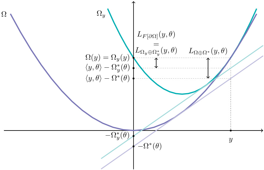
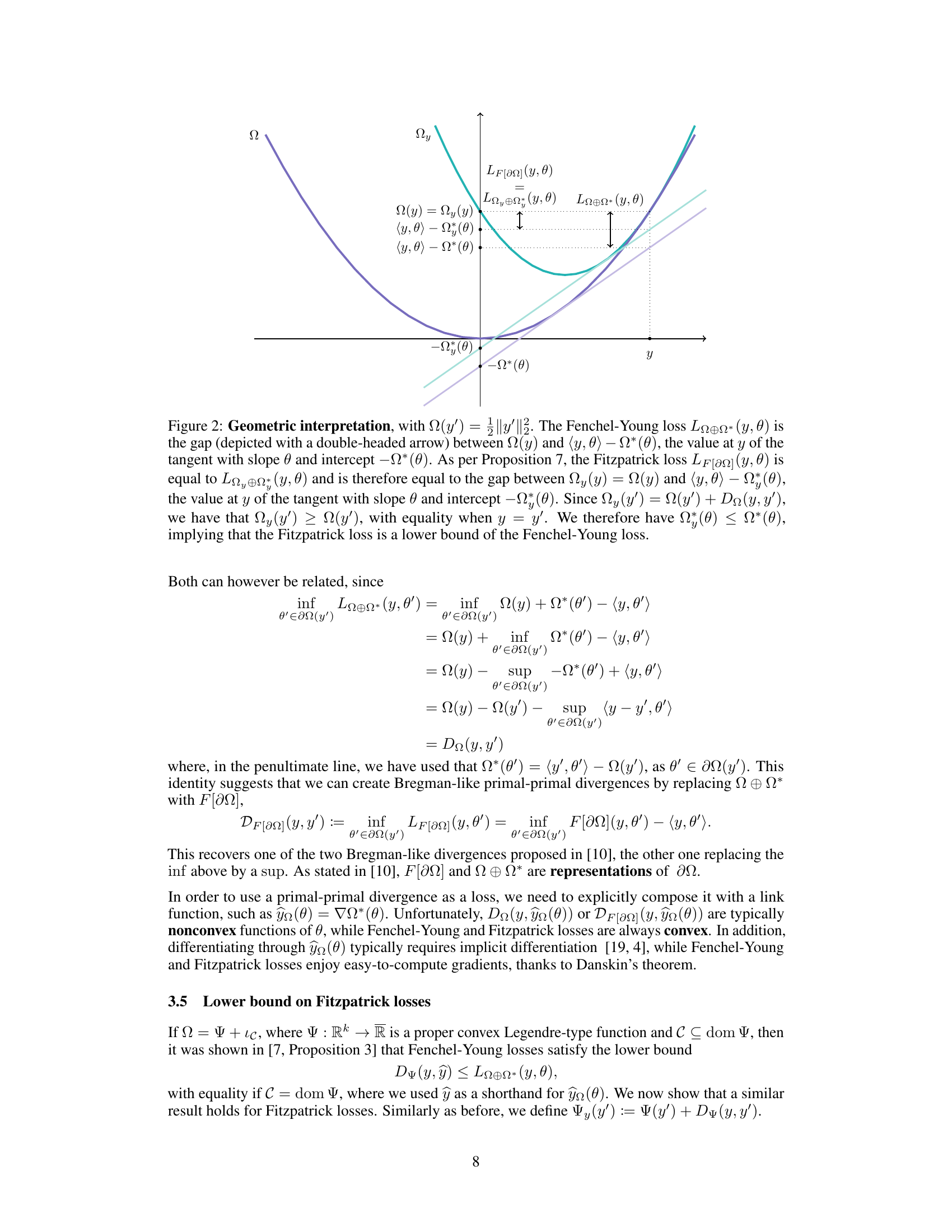
🔼 This figure illustrates the geometric relationship between Fenchel-Young losses and Fitzpatrick losses. It shows that the Fitzpatrick loss is always lower than or equal to the Fenchel-Young loss, for a given convex function Ω. This relationship is demonstrated using the squared 2-norm function, showing how the gap between the function and its tangent line represents the loss, with the Fitzpatrick loss being a tighter bound than the Fenchel-Young loss.
read the caption
Figure 2: Geometric interpretation, with Ω(y') = ½||y' ||2. The Fenchel-Young loss LΩ⊕Ω*(y, θ) is the gap (depicted with a double-headed arrow) between Ω(y) and 〈y, θ〉 – Ω*(θ), the value at y of the tangent with slope θ and intercept –Ω*(θ). As per Proposition 7, the Fitzpatrick loss LF[∂Ω](y, θ) is equal to LΩy⊕Ω*(y, θ) and is therefore equal to the gap between Ωy(y) = Ω(y) and 〈y, θ〉 – Ω*(θ), the value at y of the tangent with slope θ and intercept –Ω*(θ). Since Ωy(y') = Ω(y') + DΩ(y, y'), we have that Ωy(y') ≥ Ω(y'), with equality when y = y'. We therefore have Ω*(θ) ≤ Ω*(θ), implying that the Fitzpatrick loss is a lower bound of the Fenchel-Young loss.
More on tables

🔼 This table compares the performance of four different loss functions (sparsemax, Fitzpatrick sparsemax, logistic, and Fitzpatrick logistic) on eleven multi-label datasets. The performance metric is mean squared error (MSE), which measures the difference between predicted and true label proportions. Bold values indicate a significant improvement (at least 0.005 MSE) of a Fitzpatrick loss over its corresponding standard loss function.
read the caption
Table 1: Test performance comparison between the sparsemax loss, the logistic loss and their Fitzpatrick counterparts on the task of label proportion estimation, with regularization parameter λ tuned against the validation set. For each dataset, label proportion errors are measured using the mean squared error (MSE). We use bold if the error is at least 0.005 lower than its counterpart.

🔼 This table compares the performance of four different loss functions (sparsemax, Fitzpatrick sparsemax, logistic, and Fitzpatrick logistic) on eleven different datasets for the task of label proportion estimation. The performance metric is mean squared error (MSE), and bold values indicate an MSE improvement of at least 0.005 compared to the corresponding non-Fitzpatrick loss.
read the caption
Table 1: Test performance comparison between the sparsemax loss, the logistic loss and their Fitzpatrick counterparts on the task of label proportion estimation, with regularization parameter λ tuned against the validation set. For each dataset, label proportion errors are measured using the mean squared error (MSE). We use bold if the error is at least 0.005 lower than its counterpart.

🔼 This table compares the performance of four different loss functions: sparsemax loss, Fitzpatrick sparsemax loss, logistic loss, and Fitzpatrick logistic loss. The comparison is done on eleven different datasets, with the performance metric being the mean squared error (MSE) of label proportion estimation. The results show that the Fitzpatrick losses sometimes offer slightly better results than their Fenchel-Young counterparts, but the differences are small and not consistently favorable to the Fitzpatrick losses.
read the caption
Table 1: Test performance comparison between the sparsemax loss, the logistic loss and their Fitzpatrick counterparts on the task of label proportion estimation, with regularization parameter λ tuned against the validation set. For each dataset, label proportion errors are measured using the mean squared error (MSE). We use bold if the error is at least 0.005 lower than its counterpart.
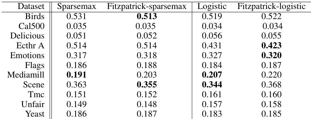
🔼 This table presents a comparison of the performance of four different loss functions on eleven multi-label classification datasets. The loss functions compared are the standard sparsemax and logistic losses, along with their corresponding Fitzpatrick loss counterparts. Performance is measured by the mean squared error (MSE) of label proportion estimates. The bold values indicate cases where the Fitzpatrick loss shows an improvement of at least 0.005 MSE compared to its standard counterpart.
read the caption
Table 1: Test performance comparison between the sparsemax loss, the logistic loss and their Fitzpatrick counterparts on the task of label proportion estimation, with regularization parameter λ tuned against the validation set. For each dataset, label proportion errors are measured using the mean squared error (MSE). We use bold if the error is at least 0.005 lower than its counterpart.
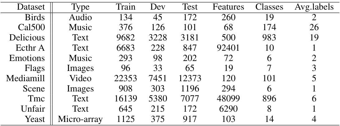
🔼 This table presents the statistics of eleven benchmark datasets used in the experiments section of the paper. For each dataset, it provides information on the type of data (e.g., audio, music, text, images, video, microarray), the number of training, development, and test samples, the number of features, the number of classes, and the average number of labels per sample.
read the caption
Table 2: Datasets statistics

🔼 This table compares the performance of four different loss functions (Sparsemax, Fitzpatrick sparsemax, Logistic, and Fitzpatrick logistic) on eleven multi-label datasets in terms of mean squared error (MSE). The regularization parameter (λ) was tuned via cross-validation. Bold values indicate that the MSE is at least 0.005 lower than the corresponding loss function without the Fitzpatrick refinement.
read the caption
Table 1: Test performance comparison between the sparsemax loss, the logistic loss and their Fitzpatrick counterparts on the task of label proportion estimation, with regularization parameter λ tuned against the validation set. For each dataset, label proportion errors are measured using the mean squared error (MSE). We use bold if the error is at least 0.005 lower than its counterpart.

🔼 This table compares the performance of four different loss functions for label proportion estimation across eleven datasets. The loss functions are the standard sparsemax and logistic losses, and their counterparts using the newly proposed Fitzpatrick loss. Mean squared error (MSE) is used as the performance metric, and bold values indicate where a Fitzpatrick loss outperforms its standard equivalent by at least a margin of 0.005.
read the caption
Table 1: Test performance comparison between the sparsemax loss, the logistic loss and their Fitzpatrick counterparts on the task of label proportion estimation, with regularization parameter λ tuned against the validation set. For each dataset, label proportion errors are measured using the mean squared error (MSE). We use bold if the error is at least 0.005 lower than its counterpart.
Full paper#
