TL;DR#
Hippocampal place cells, crucial for spatial navigation, exhibit remapping—changing their firing patterns based on context. Existing models struggle to replicate this complex behavior. This paper addresses this by proposing a novel similarity-based objective function to train neural networks. The objective leverages proximity in space to learn similar representations, and is easily extended to incorporate context.
The trained network successfully replicates place cell-like representations and context-dependent remapping. This suggests that spatial representations in biological systems may emerge from a similarity-based principle. The network also displays orthogonal invariance, generating new representations through transformations without explicit re-learning, similar to biological remapping. This innovative approach sheds light on the formation and encoding mechanisms of place cells and provides a new perspective on representational reuse in neural systems.
Key Takeaways#
Why does it matter?#
This paper is crucial for researchers in neuroscience and AI because it introduces a novel, biologically-inspired objective function that enables the learning of place cell-like representations in neural networks. This opens new avenues for understanding spatial navigation, memory encoding, and developing more biologically plausible AI models. The research is relevant to the current trends in self-supervised learning and neural network architectures for spatial tasks.
Visual Insights#

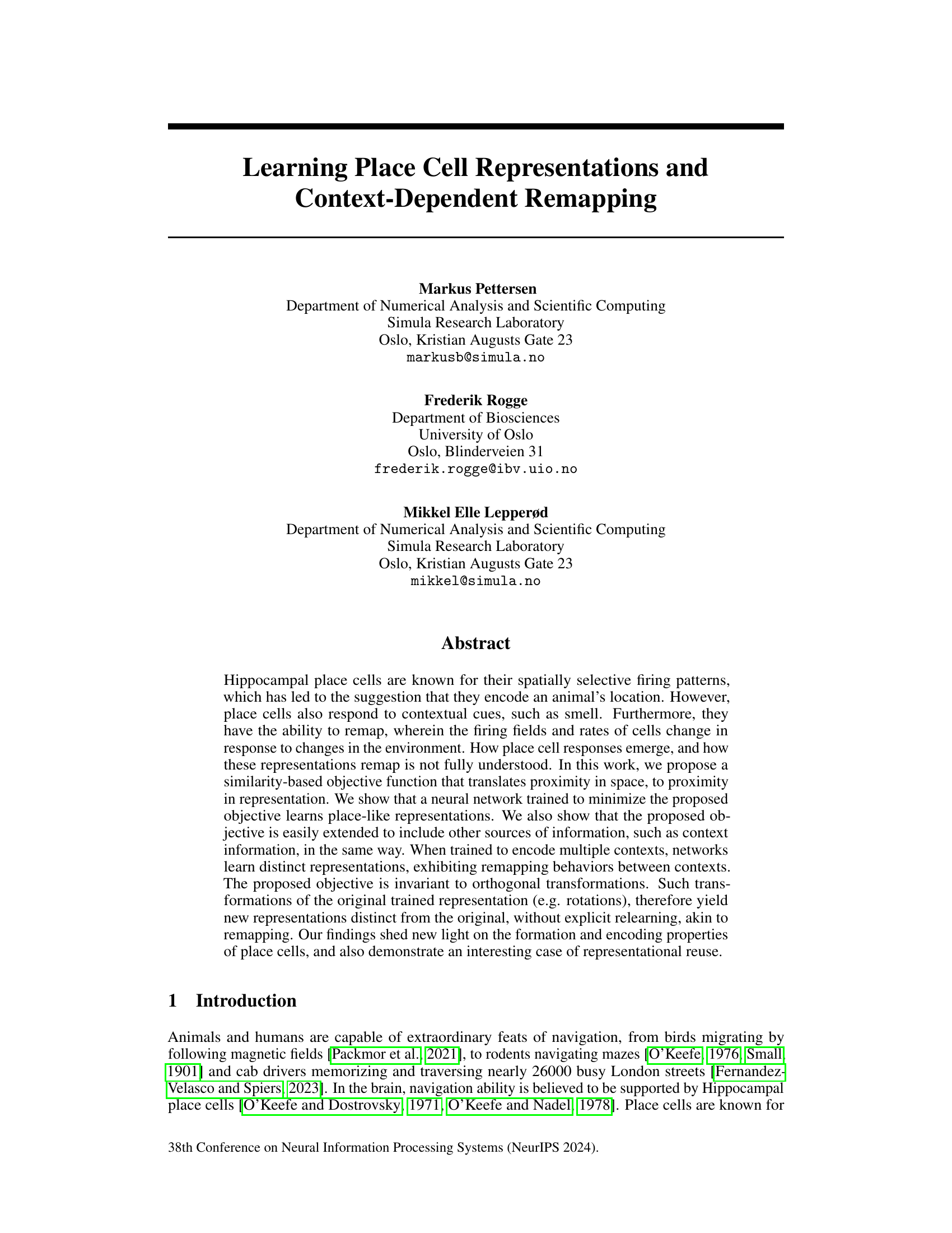
🔼 This figure provides a visual overview of the models and objectives used in the study. Panel (a) illustrates the core concept of the spatial objective function: nearby locations should have similar neural representations, while distant locations should have dissimilar representations. Panel (b) extends this concept to include contextual information, showing that similar contexts should also have similar representations. Panel (c) combines both spatial and contextual information, demonstrating that the model can learn joint representations of space and context. Finally, panel (d) shows example ratemaps (a visualization of neural activity) from both a recurrent neural network (RNN) and a feedforward neural network (FF) trained to minimize the spatial objective function. These ratemaps show the spatial selectivity of the neurons, illustrating the emergence of place-like representations.
read the caption
Figure 1: Overview of models and objective. a) Illustration of the spatial objective: locations that are close should be encoded by similar population vectors, distant locations by dissimilar population vectors. b) Similar to a); similar context signals should be represented by similar population vectors, dissimilar contexts by dissimilar population vectors. c) Similar to a) and b), but for joint encoding of space and context. d) Ratemaps of randomly selected units in networks trained to minimize the spatial objective function. Shown are learned representations for a recurrent network performing simultaneous path integration, and a feedforward network performing spatial encoding.
In-depth insights#
Spatial Encoding#
Spatial encoding in the context of hippocampal place cells is a fascinating area of neuroscience. The paper investigates how the brain translates spatial proximity into representational proximity, proposing a similarity-based objective function for a neural network. This approach successfully learns place-like representations, demonstrating the network’s ability to encode spatial information by associating nearby locations with similar neural activations. A key finding is the objective’s adaptability, allowing the incorporation of other information sources such as context, which is essential for understanding how the brain handles context-dependent remapping. The invariance to orthogonal transformations (e.g., rotations) suggests a robust and flexible internal representation of space, implying that remapping might not require extensive relearning, but rather the application of these transformations to existing representations. Overall, the work provides a novel theoretical framework with significant implications for future research on spatial cognition and neural network models of the hippocampus.
Contextual Remapping#
The concept of “Contextual Remapping” in hippocampal place cells refers to the dynamic adjustment of spatial representations based on environmental context. Place cells, which fire selectively in specific locations, exhibit different firing patterns across contexts, even in the same physical environment. This remapping isn’t simply noise but a flexible adaptation mechanism that allows the brain to distinguish between different experiences. The underlying neural mechanisms remain an area of active research, but computational models suggest that context influences the weighting of various inputs leading to distinct, context-specific spatial representations. This adaptability is crucial for navigation and memory because it enables the brain to create distinct, context-rich memories that are not easily confused. The study of contextual remapping provides critical insights into the brain’s remarkable ability to encode and retrieve spatial information flexibly. Importantly, understanding how this process works is pivotal to developing more sophisticated artificial navigation and memory systems.
Network Architectures#
The research paper explores the use of neural networks to model hippocampal place cells, focusing on learning spatial representations. Two main network architectures are investigated: feedforward and recurrent. The feedforward network, a simpler model, is used to establish the core principles of the proposed similarity-based objective function, demonstrating its effectiveness in learning place-like representations. This simplicity allows for easier analysis of the learned spatial features. The recurrent network, on the other hand, provides a more biologically realistic and complex model, capable of incorporating path integration. This architecture enables the study of both place and band cell representations, offering richer insights into the interplay of spatial coding mechanisms. The choice between these architectures highlights a trade-off between analytical tractability and biological realism. The feedforward model aids in understanding fundamental aspects while the recurrent network extends the model to capture the dynamic and sequential nature of spatial navigation. The selection of these architectures is strategic, aiming to thoroughly examine both the theoretical foundation and biological relevance of the proposed learning objective.
Orthogonal Transforms#
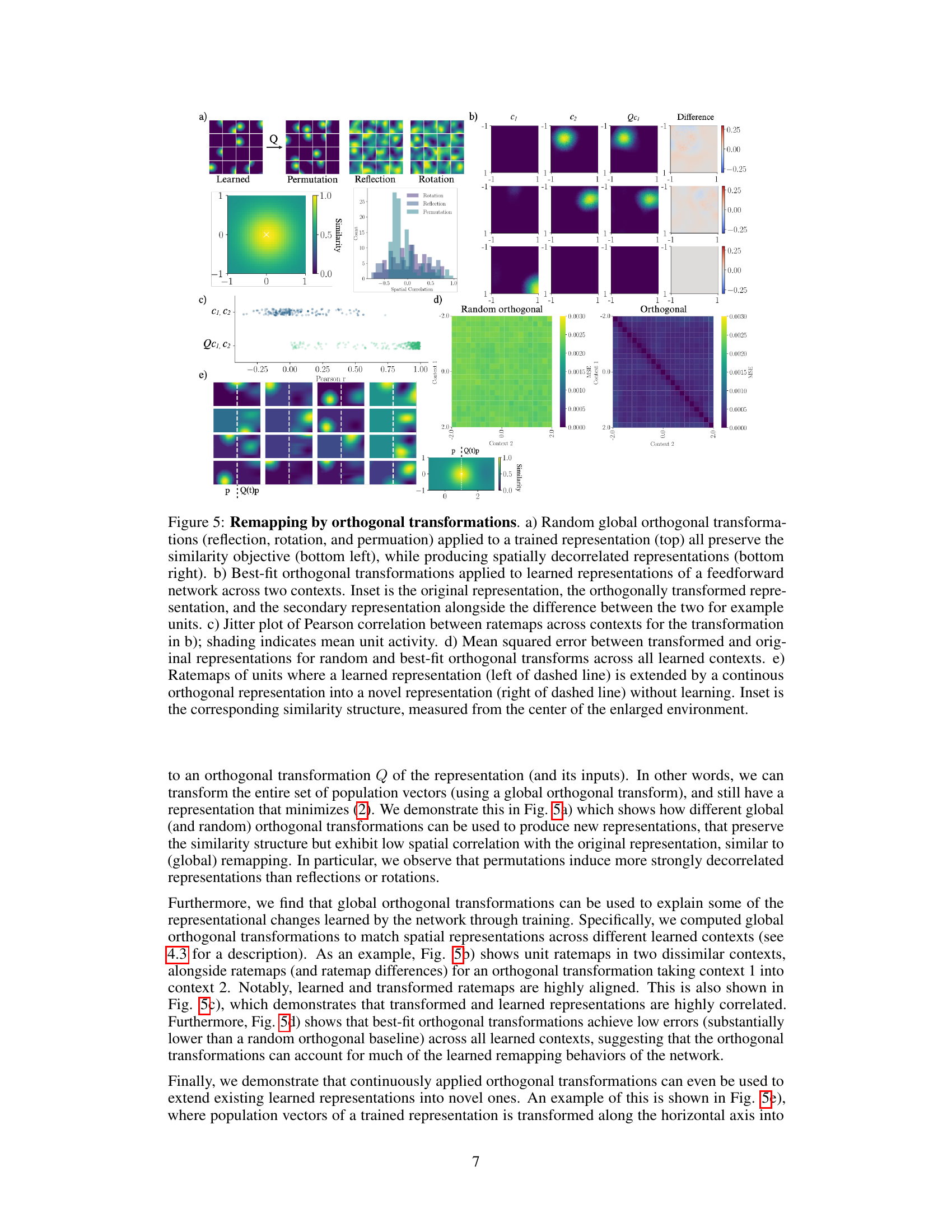
The concept of orthogonal transformations within the context of learning spatial representations offers a fascinating approach to understanding hippocampal remapping. The research leverages the invariance of the objective function to orthogonal transformations to demonstrate how new, distinct spatial representations can be generated from an existing representation without retraining. This process mimics the observed behavior of place cells in biological systems, exhibiting remapping without explicit relearning. This suggests a mechanistic explanation for remapping that relies on transforming existing internal representations rather than learning entirely new ones. The study further explores the impact of different orthogonal transformations (rotation, reflection, permutation), revealing that they produce varying degrees of decorrelation between the original and transformed representations. This finding sheds light on the flexibility and complexity of hippocampal spatial encoding and its potential adaptation to changing environments. The ability to generate novel maps through simple transformations, rather than extensive re-training, provides an efficient and biologically plausible mechanism for dynamic spatial representation and context-dependent learning.
Future Directions#
Future research could explore several promising avenues. Extending the model to handle more complex contextual information, beyond scalar signals, is crucial for better biological realism. This could involve incorporating spatial context or multiple contextual cues simultaneously. Investigating alternative similarity measures and distance functions beyond the Gaussian and Euclidean metrics used here might reveal novel representational properties. Exploring different network architectures, such as spiking neural networks, could provide further insight into how place cell-like representations emerge in biological systems. Finally, directly comparing model predictions with experimental data from place cell recordings is essential to validate the model’s biological plausibility and uncover potential limitations. This comparative analysis will reveal how well the model captures the nuanced dynamics of hippocampal remapping and inform future model refinements.
More visual insights#
More on figures

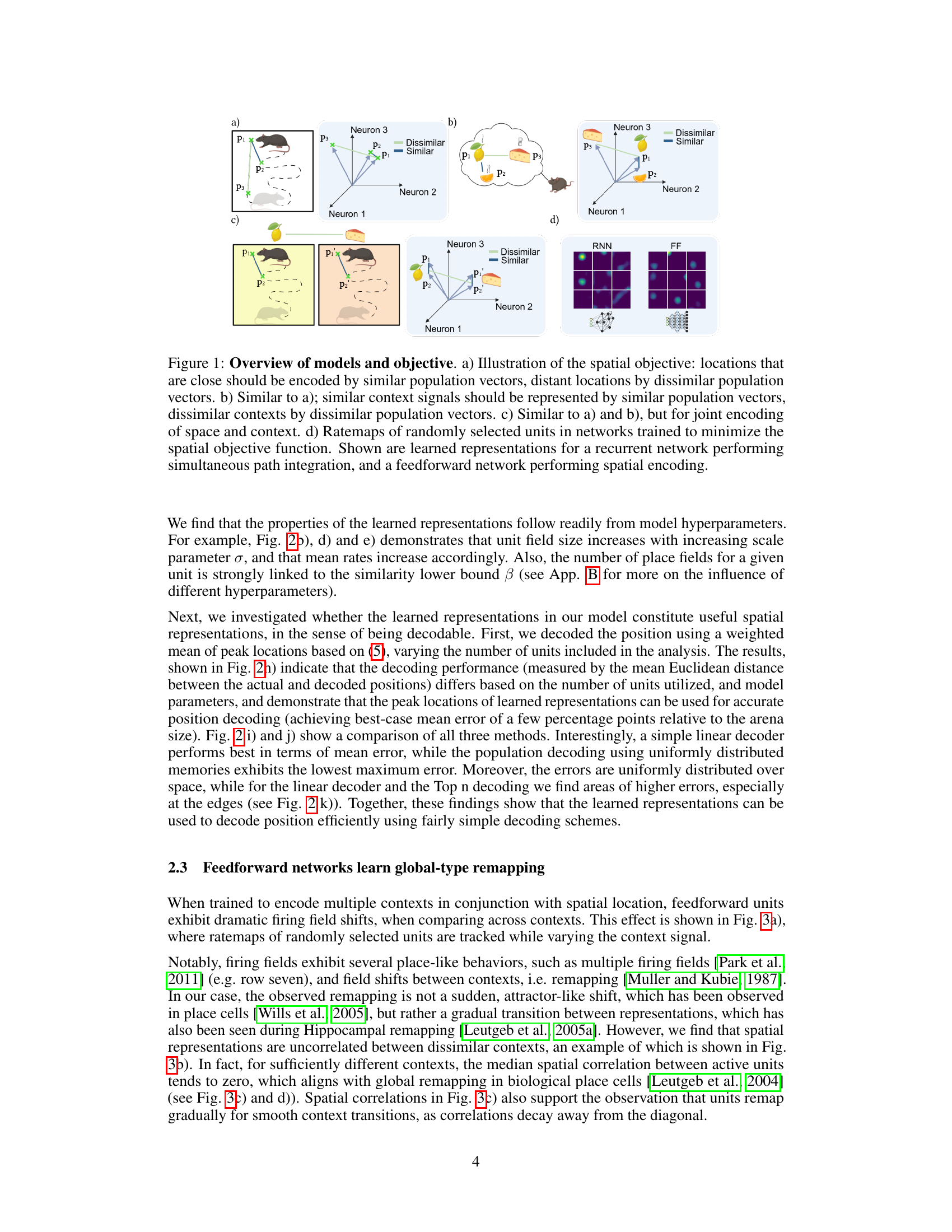
🔼 This figure shows the results of training a feedforward network using the similarity-based objective function. It demonstrates how different hyperparameters affect the learned representations, including the training loss, the spatial tuning of the units (ratemaps), the proportion of active units, and the accuracy of position decoding. The figure also compares the similarity structure between the target and the learned representations.
read the caption
Figure 2: Feedforward network results. a) Training loss for different parameter combinations. Line shows the mean of 10 models and error bands show the min and max across models. Note that training data is generated continuously. b) Example ratemaps of randomly selected active units for models with different scale parameters σ. Color scale is relative to individual unit activity. c) Distributions of the proportion of active units (mean rate > 0) for different parameter combinations across 10 models. d) Distribution of mean rate of units for each parameter combination (shown for one example model each). e) Field sizes in pixels for each parameter combination (shown for one example model each). f) Left: Example target similarity structure relative to center. Middle: corresponding similarity for the learned representations of model with σ = 0.25 and β = 0.5. Right: difference between target and learned similarity. g) Peak locations of all units for different parameter combinations (shown for one example model each). h) Mean position decoding error as a function of the number of units used for Top n decoding. Dashed line shows the naive case where every decoded position is at the center. i) and j) Mean and max decoding error for different decoding methods for trained 10 models, each with σ = 0.25 and β = 0.5. k) Example decoding error maps for different decoding methods (σ = 0.25 and β = 0.5).

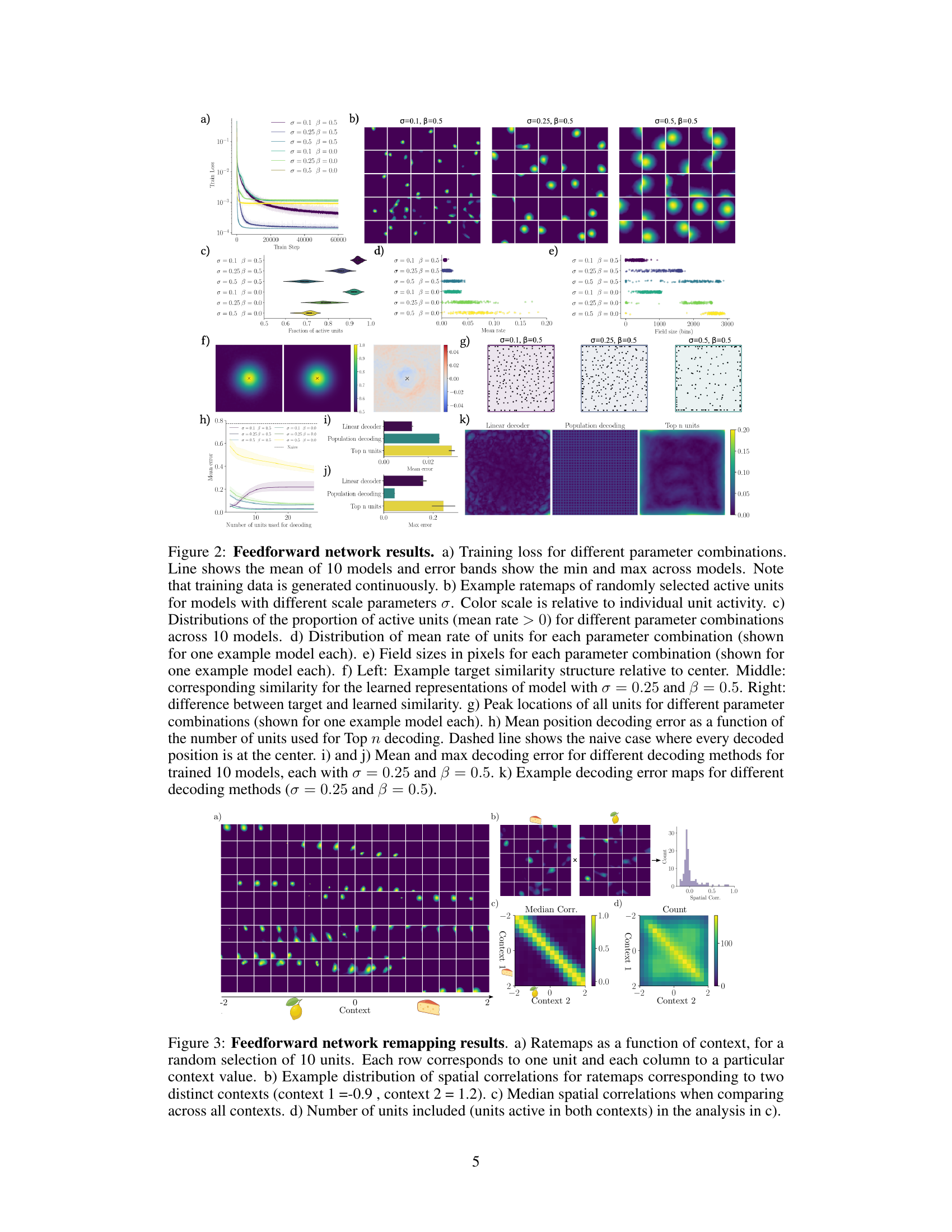
🔼 This figure demonstrates the remapping behavior of feedforward networks trained to encode multiple contexts. Panel (a) shows ratemaps (spatial tuning curves) for 10 randomly selected units across different context values. Notice how the spatial tuning changes significantly depending on the context, exhibiting global remapping. Panel (b) shows the distribution of spatial correlations between ratemaps for two specific contexts, demonstrating uncorrelated representations in different contexts. Panels (c) and (d) summarize the median spatial correlations and the number of units included in the correlation analysis across all contexts, further supporting the global remapping observation.
read the caption
Figure 3: Feedforward network remapping results. a) Ratemaps as a function of context, for a random selection of 10 units. Each row corresponds to one unit and each column to a particular context value. b) Example distribution of spatial correlations for ratemaps corresponding to two distinct contexts (context 1 =-0.9, context 2 = 1.2). c) Median spatial correlations when comparing across all contexts. d) Number of units included (units active in both contexts) in the analysis in c).
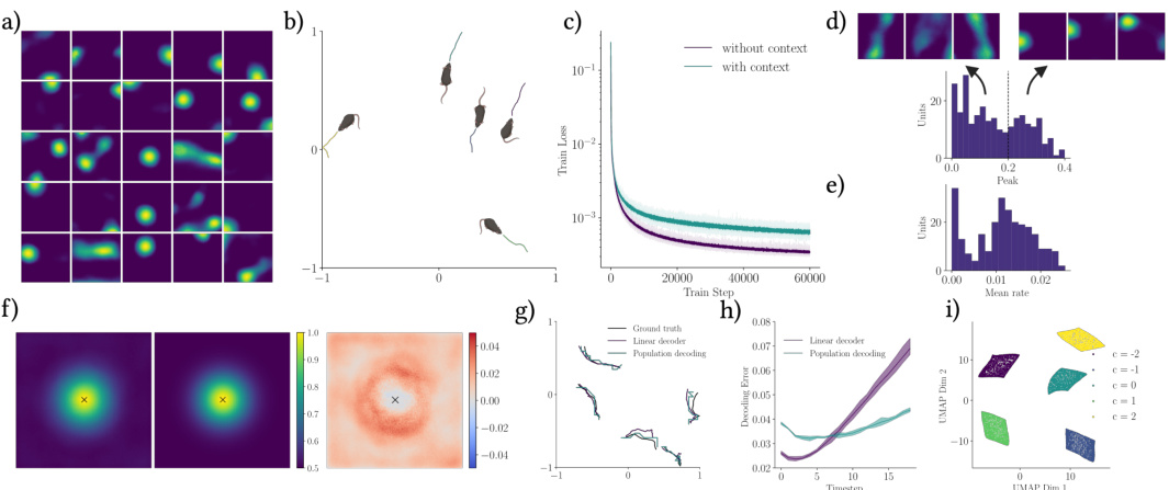
🔼 This figure shows the results of experiments using recurrent neural networks to learn spatial representations with and without context. Panel (a) displays example rate maps (spatial firing patterns) of units in a recurrent network trained without contextual information. Panel (b) shows example trajectories used during training. Panel (c) compares the training loss curves for networks trained with and without context. Panels (d) and (e) present histograms showing the distribution of peak firing rates and mean firing rates, respectively, for units in the network trained without context. Panel (f) visually compares the similarity structure of the learned representations with the target similarity structure. Panel (g) shows examples of decoded trajectories. Panel (h) compares the decoding errors from linear and population decoding methods. Finally, Panel (i) provides a 2D UMAP projection showing the spatial representations across different contexts.
read the caption
Figure 4: Recurrent network results with and without context. a) Ratemap examples of randomly selected units of a recurrent network without context. b) Example trajectories used for training. c) Training loss for recurrent networks with and without context (10 models each, error bands show min and max). d) Histogram of peak values of a recurrent network without context and example ratemaps of units of different parts of the distribution. e) Histogram of mean rates of a recurrent network without context. f) Similarity structure in the center location of the learned representations of a recurrent network without context (left) and the objective (center), as well as the difference between the two (right). g) Example trajectories decoded from network representations h) Comparison of the mean decoding error using a linear decoder or population decoding across trajectories for 10 different models each. i) 2D UMAP projection of spatial representations for different contexts.

🔼 This figure demonstrates how orthogonal transformations can be used to generate new representations that preserve the similarity structure but exhibit low spatial correlation with the original representation, similar to remapping. It shows how different global orthogonal transformations can be used to produce new representations that preserve the similarity structure but exhibit low spatial correlation with the original representation. The figure also illustrates best-fit orthogonal transformations applied to the learned representations of a feedforward network across two contexts, showing the original representation, transformed representation and the difference between them. It displays the Pearson correlation between ratemaps across contexts, the mean squared error between transformed and original representations, and demonstrates how orthogonal transformations can extend existing representations into novel ones while maintaining similarity structure.
read the caption
Figure 5: Remapping by orthogonal transformations. a) Random global orthogonal transformations (reflection, rotation, and permuation) applied to a trained representation (top) all preserve the similarity objective (bottom left), while producing spatially decorrelated representations (bottom right). b) Best-fit orthogonal transformations applied to learned representations of a feedforward network across two contexts. Inset is the original representation, the orthogonally transformed representation, and the secondary representation alongside the difference between the two for example units. c) Jitter plot of Pearson correlation between ratemaps across contexts for the transformation in b); shading indicates mean unit activity. d) Mean squared error between transformed and original representations for random and best-fit orthogonal transforms across all learned contexts. e) Ratemaps of units where a learned representation (left of dashed line) is extended by a continous orthogonal representation into a novel representation (right of dashed line) without learning. Inset is the corresponding similarity structure, measured from the center of the enlarged environment.
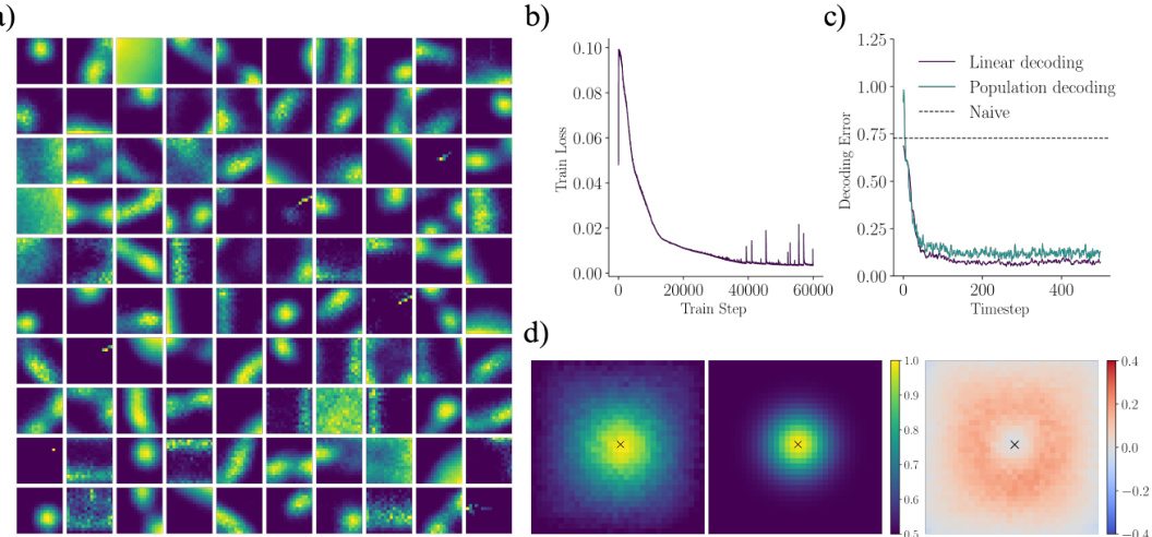
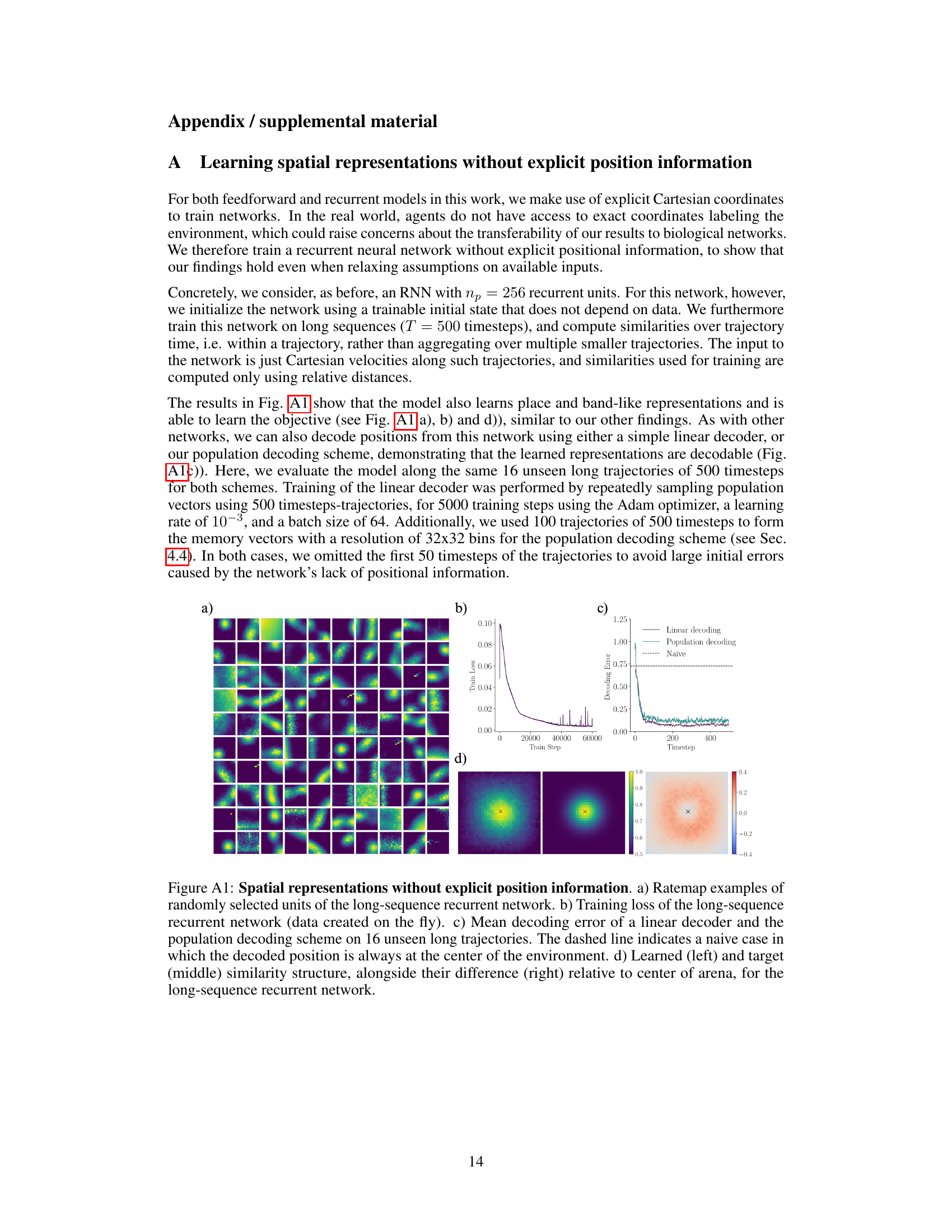
🔼 This figure shows the results of training a recurrent neural network to learn spatial representations without providing explicit position information as input. The network successfully learns place-like representations (a), minimizes the objective function over time (b), achieves accurate position decoding using both linear and population-based methods (c), and demonstrates close agreement between learned and target similarity structures (d). The results demonstrate that place-like representations can emerge even without explicit position information.
read the caption
Figure A1: Spatial representations without explicit position information. a) Ratemap examples of randomly selected units of the long-sequence recurrent network. b) Training loss of the long-sequence recurrent network (data created on the fly). c) Mean decoding error of a linear decoder and the population decoding scheme on 16 unseen long trajectories. The dashed line indicates a naive case in which the decoded position is always at the center of the environment. d) Learned (left) and target (middle) similarity structure, alongside their difference (right) relative to center of arena, for the long-sequence recurrent network.
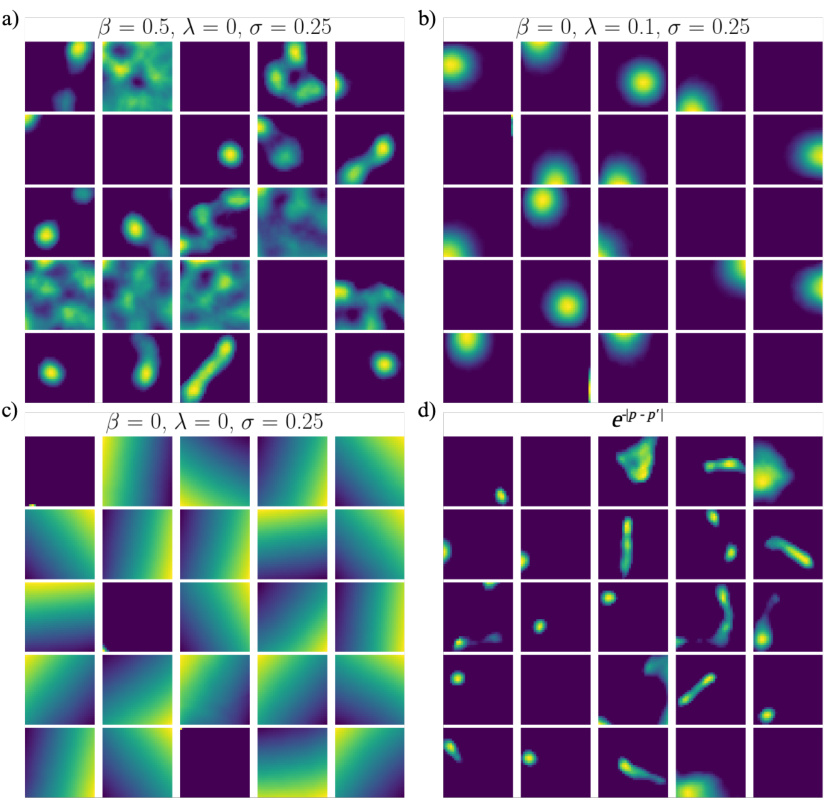
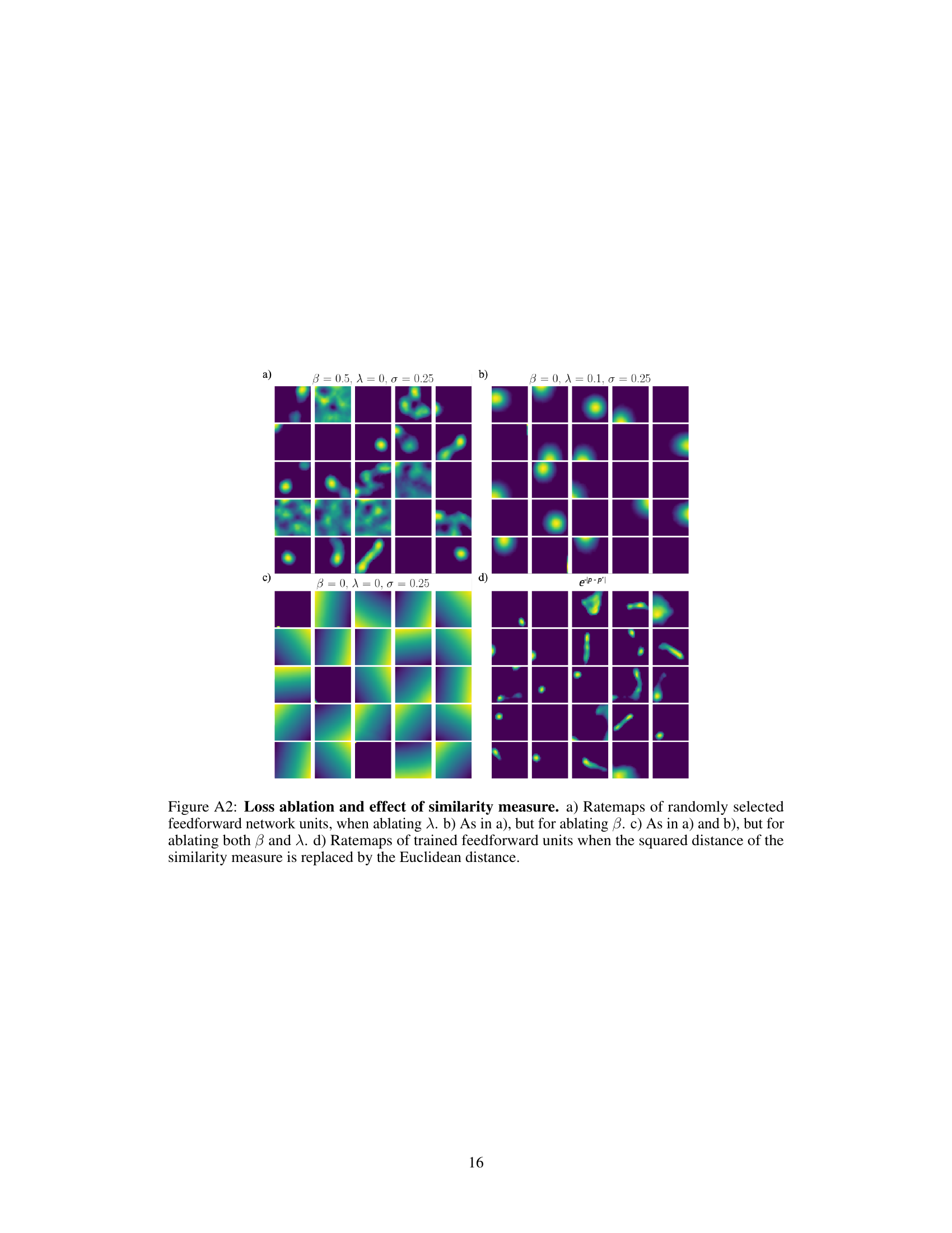
🔼 This figure shows the results of an ablation study on the hyperparameters λ and β in the loss function, as well as the impact of changing the similarity measure from Gaussian to Euclidean distance. The ablation study reveals that place-like tuning requires either a non-zero β (similarity threshold) or a non-zero λ (activity regularization). Using Euclidean distance instead of the squared Gaussian distance maintains place-like tuning but results in more variable field sizes.
read the caption
Figure A2: Loss ablation and effect of similarity measure. a) Ratemaps of randomly selected feedforward network units, when ablating λ. b) As in a), but for ablating β. c) As in a) and b), but for ablating both β and λ. d) Ratemaps of trained feedforward units when the squared distance of the similarity measure is replaced by the Euclidean distance.

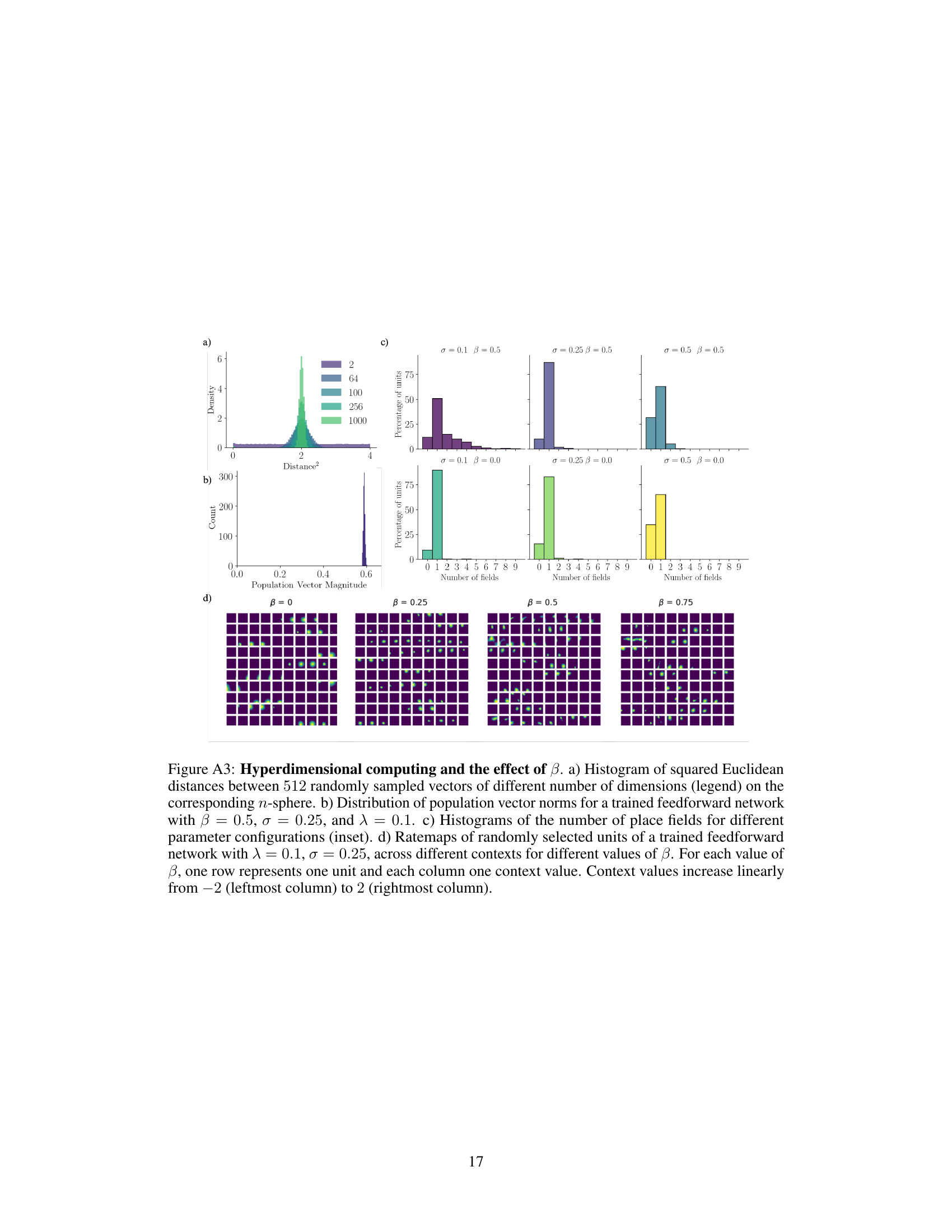
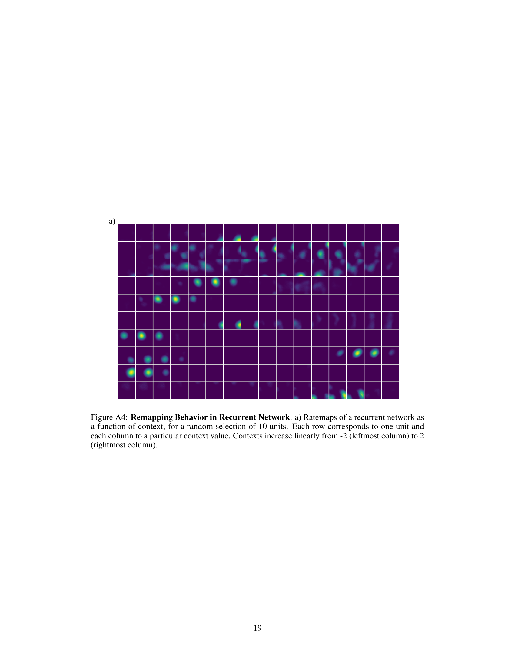
🔼 Figure A3 shows the effect of the hyperparameter β on the learned representation. Panel (a) demonstrates that high-dimensional vectors tend to be equidistant from one another. Panel (b) shows the distribution of population vector magnitudes for a trained network, demonstrating that most vectors have magnitudes near 1. Panel (c) illustrates the effect of β and σ on the number of place fields per unit, and panel (d) presents a set of ratemaps demonstrating how increasing β leads to more robust remapping across contexts.
read the caption
Figure A3: Hyperdimensional computing and the effect of β. a) Histogram of squared Euclidean distances between 512 randomly sampled vectors of different number of dimensions (legend) on the corresponding n-sphere. b) Distribution of population vector norms for a trained feedforward network with β = 0.5, σ = 0.25, and λ = 0.1. c) Histograms of the number of place fields for different parameter configurations (inset). d) Ratemaps of randomly selected units of a trained feedforward network with λ = 0.1, σ = 0.25, across different contexts for different values of β. For each value of β, one row represents one unit and each column one context value. Context values increase linearly from -2 (leftmost column) to 2 (rightmost column).
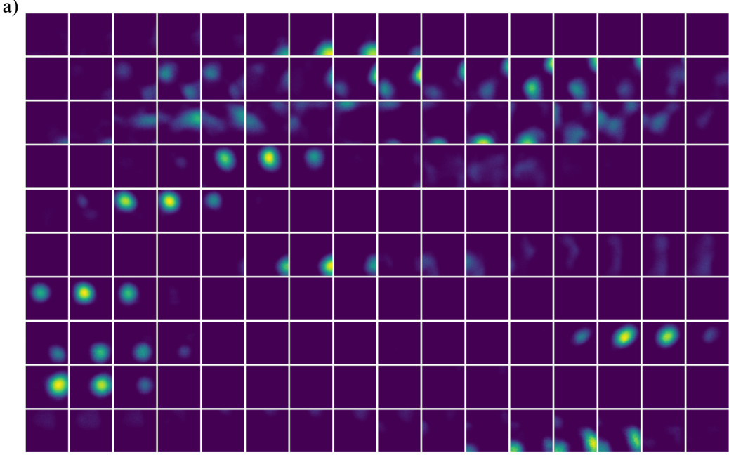
🔼 This figure demonstrates that even without explicit position information provided to the network, the recurrent network can still learn spatial representations similar to place cells. It displays rate maps (spatial firing patterns of neurons), training loss curves, decoding error plots (comparing the network’s estimated location to the actual location), and a comparison of the learned and target similarity structures. The results show that the network successfully minimizes the similarity-based objective function and learns representations that are both place-like and decodable, highlighting the robustness of the proposed approach even under less constrained input conditions.
read the caption
Figure A1: Spatial representations without explicit position information. a) Ratemap examples of randomly selected units of the long-sequence recurrent network. b) Training loss of the long-sequence recurrent network (data created on the fly). c) Mean decoding error of a linear decoder and the population decoding scheme on 16 unseen long trajectories. The dashed line indicates a naive case in which the decoded position is always at the center of the environment. d) Learned (left) and target (middle) similarity structure, alongside their difference (right) relative to center of arena, for the long-sequence recurrent network.
Full paper#
