TL;DR#
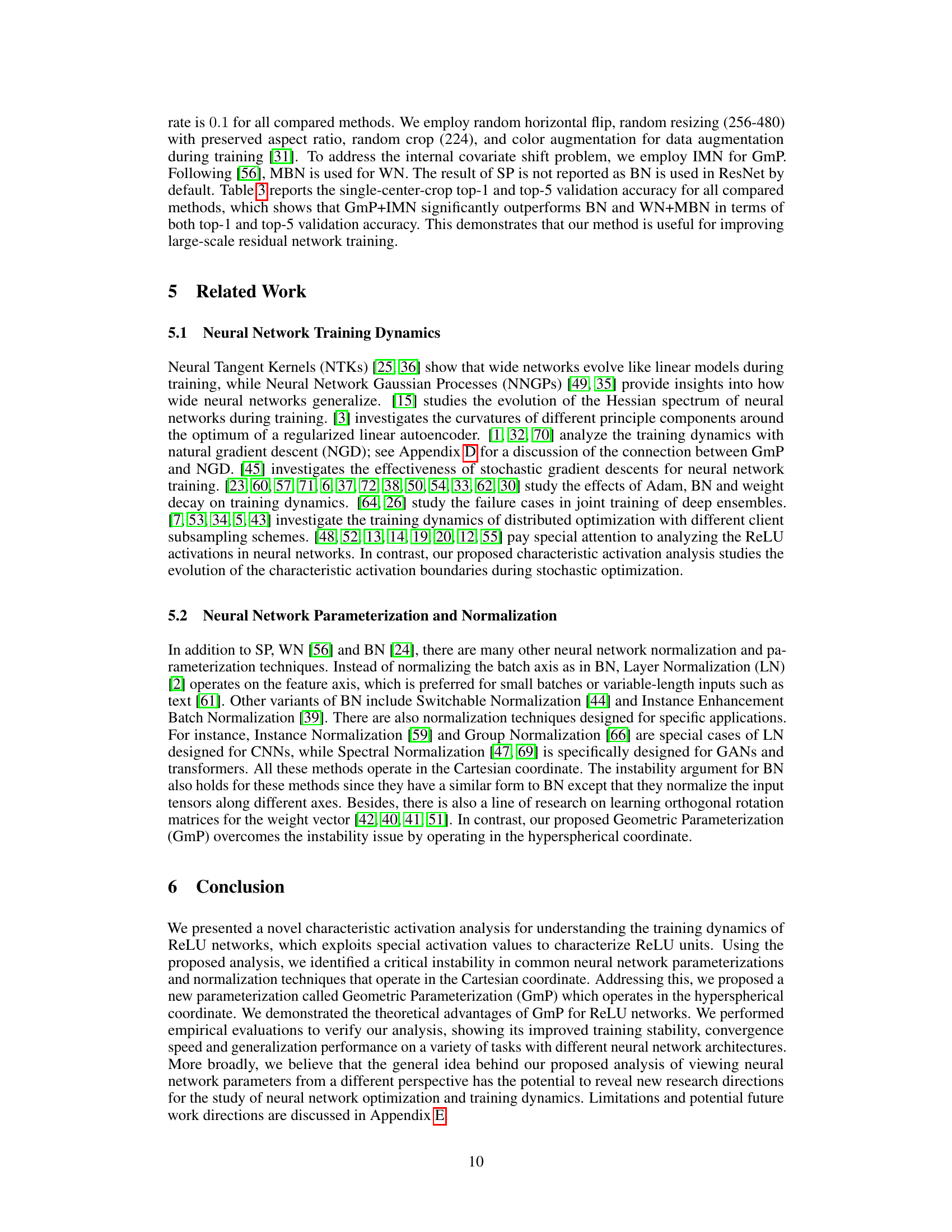
Many common neural network parameterizations suffer from instability during training, hindering fast convergence and good generalization. This instability stems from issues in how these parameterizations handle the characteristic activation boundaries of ReLU neurons. These boundaries define the regions where neurons switch between active and inactive states. The paper identifies how stochastic optimization methods disrupt the boundaries, impacting training performance.
To overcome this, the authors propose Geometric Parameterization (GmP). GmP uses a hyperspherical coordinate system to parameterize neural network weights, effectively separating radial and angular components. This disentanglement stabilizes the characteristic activation boundaries during training. Experiments show that GmP significantly improves optimization stability, accelerates convergence, and enhances the generalization ability of various neural network models, demonstrating its effectiveness on multiple benchmarks.
Key Takeaways#
Why does it matter?#
This paper is highly important for researchers working on neural network optimization and training dynamics. It addresses a critical instability issue in common neural network parameterizations, offering a novel solution—Geometric Parameterization (GmP)—that significantly improves optimization stability, convergence speed, and generalization performance. The findings are relevant to various deep learning applications, opening new avenues for research in neural network design and training strategies. The theoretical analysis and empirical results provide valuable insights for improving the efficiency and effectiveness of training deep neural networks.
Visual Insights#

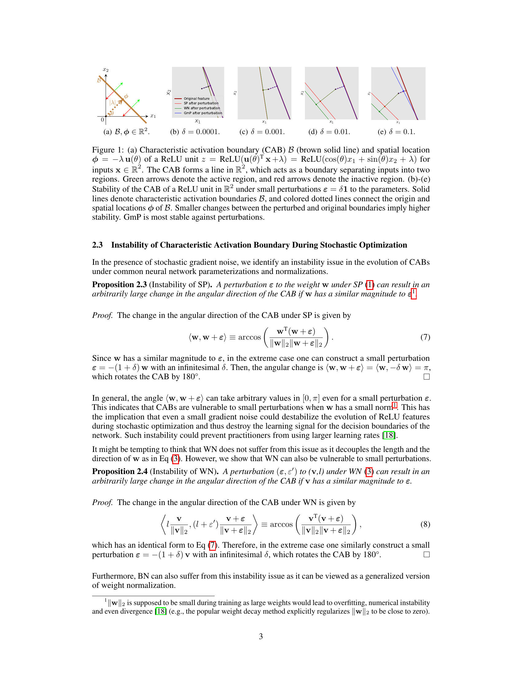
🔼 This figure illustrates the characteristic activation boundary (CAB) and its spatial location for a ReLU unit. Subfigures (a) shows the CAB as a line separating active and inactive regions in a 2D input space. Subfigures (b) through (e) demonstrate the stability of the CAB under small parameter perturbations for different parameterization methods (SP, WN, GmP). GmP shows significantly higher stability.
read the caption
Figure 1: (a) Characteristic activation boundary (CAB) B (brown solid line) and spatial location φ = −λu(θ) of a ReLU unit z = ReLU(u(θ)x+λ) = ReLU(cos(θ)x₁ + sin(θ)x₂ + λ) for inputs x ∈ R². The CAB forms a line in R², which acts as a boundary separating inputs into two regions. Green arrows denote the active region, and red arrows denote the inactive region. (b)-(e) Stability of the CAB of a ReLU unit in R² under small perturbations ε = δι to the parameters. Solid lines denote characteristic activation boundaries B, and colored dotted lines connect the origin and spatial locations φ of B. Smaller changes between the perturbed and original boundaries imply higher stability. GmP is most stable against perturbations.

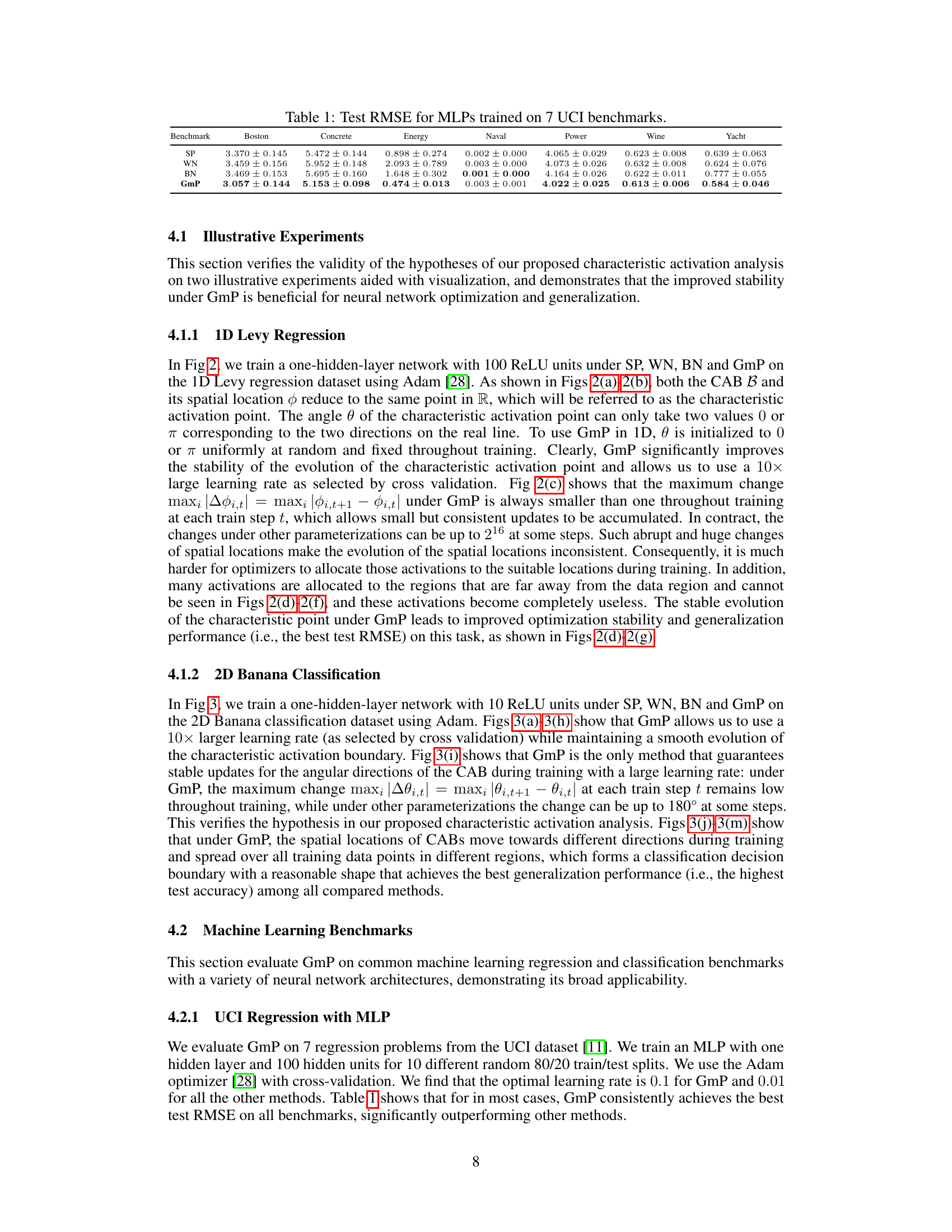
🔼 This table presents the test root mean squared error (RMSE) achieved by four different neural network parameterization methods (SP, WN, BN, and GmP) on seven regression datasets from the UCI machine learning repository. Lower RMSE values indicate better performance. The results show that GmP generally outperforms the other methods across most datasets.
read the caption
Table 1: Test RMSE for MLPs trained on 7 UCI benchmarks.
In-depth insights#
ReLU Instability#
The ReLU instability issue, central to the paper, highlights a critical vulnerability in common neural network training practices. Standard parameterizations, like weight normalization and batch normalization, fail to effectively decouple weight magnitude and direction, leading to instability in the characteristic activation boundaries of ReLU units. These boundaries, crucial for decision-making, become highly sensitive to the inherent noise of stochastic gradient descent, impeding convergence and generalization. This instability is not simply a minor nuisance; it directly impacts optimization performance and model generalization. The analysis powerfully demonstrates that the Cartesian coordinate systems used in conventional methods are fundamentally unsuitable for robust ReLU training. In contrast, the paper advocates for geometric parameterization, which leverages the hyperspherical coordinate system to elegantly separate radial and angular weight components. This elegant solution stabilizes the dynamics of the activation boundaries, resulting in faster convergence, improved generalization, and overall enhanced training stability. The empirical results strongly confirm this theoretical advantage, making geometric parameterization a significant contribution towards more robust and efficient deep learning.
GmP Parameterization#
The proposed Geometric Parameterization (GmP) offers a novel approach to addressing instability issues in training ReLU networks. GmP leverages a hyperspherical coordinate system, effectively separating the radial and angular components of weight vectors. This decoupling is crucial because it mitigates the instability observed in standard parameterizations (like SP, WN, and BN) where even small perturbations can significantly alter activation boundaries. Theoretically, GmP stabilizes the evolution of characteristic activation boundaries, enhancing training stability and potentially improving generalization. Empirical results showcase significant improvements in optimization stability, convergence speed, and generalization performance across various models and benchmarks, strongly supporting the theoretical claims and demonstrating the practical advantages of GmP for training deep ReLU networks.
Hyperspherical Stability#
Hyperspherical stability, in the context of neural networks, likely refers to a method of parameterization that enhances the robustness of training by leveraging the properties of hyperspheres. Standard parameterizations in Cartesian coordinates are susceptible to instability during stochastic gradient descent, causing erratic updates and hindering convergence. A hyperspherical approach might use spherical coordinates to represent weights, decoupling the magnitude (radius) and direction (angles) of the weight vector. This separation can stabilize the training dynamics, reducing sensitivity to noise and leading to more reliable and efficient learning. The theoretical underpinnings would likely show that small perturbations in the hyperspherical representation result in bounded changes to the activation boundaries, unlike Cartesian approaches which can exhibit unbounded changes. Empirical evaluations would then demonstrate this enhanced stability through faster convergence speeds and improved generalization performance across various datasets and network architectures. In essence, hyperspherical stability offers a novel approach to addressing inherent challenges in neural network training, promising improved robustness and efficiency.
Empirical Validation#
An empirical validation section in a research paper would rigorously test the proposed methods. It should present results on diverse, challenging datasets, comparing performance against established baselines. Detailed experimental setups and hyperparameter choices need to be clearly described for reproducibility. Ideally, the validation would involve multiple metrics relevant to the problem, going beyond just accuracy. Statistical significance should be assessed, with error bars or p-values to indicate the reliability of the findings. The discussion should interpret results thoughtfully, addressing limitations and exploring potential reasons for observed successes or failures. Visualizations are important to communicate results effectively, especially for complex models. The strength of the validation relies heavily on the breadth and depth of the tests, demonstrating the proposed method’s robustness and generalizability.
Future Directions#
The paper’s core contribution is introducing Geometric Parameterization (GmP) to stabilize neural network training. Future research could explore extending GmP beyond ReLU activations to encompass other activation functions like sigmoid, tanh, or other piecewise linear functions. A key limitation is the current focus on single-hidden-layer networks. Scaling the analysis and GmP’s effectiveness to deeper networks is crucial for broader impact. Investigating the effect of GmP on large-width networks is also important, examining how it interacts with the neural tangent kernel (NTK) regime. Understanding its interaction with other normalization techniques like batch normalization (BN) or layer normalization (LN) would enrich its practical applicability. Theoretical investigation of GmP’s limiting behavior in high dimensions could provide further theoretical guarantees. Finally, experimenting with different initialization strategies and exploring the impact of GmP on the efficiency of optimization algorithms would be valuable future directions.
More visual insights#
More on figures
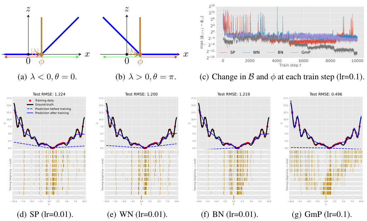
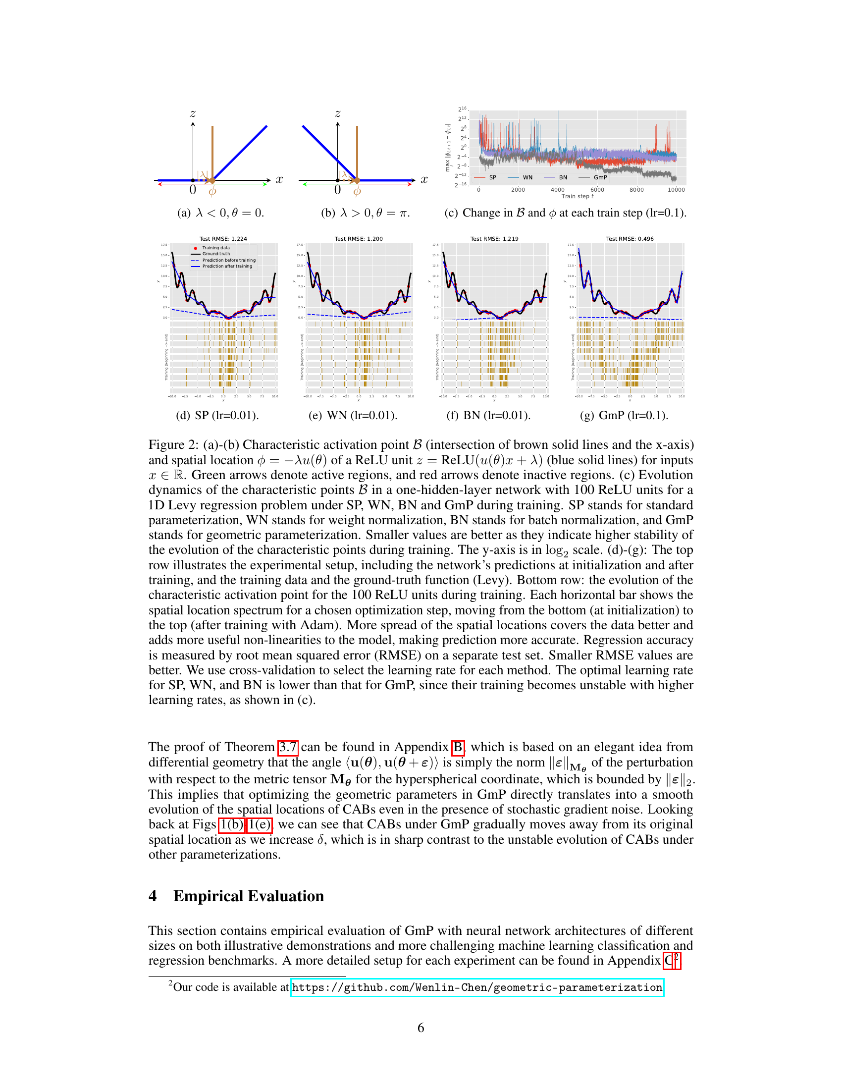
🔼 This figure shows the characteristic activation point and its evolution during training for different parameterizations (SP, WN, BN, GmP). It illustrates how GmP leads to more stable training and better generalization performance in a 1D Levy regression task by maintaining a consistent movement of activation points during training. The figure highlights the instability of SP, WN, and BN, showing that they can have erratic behavior resulting in less optimal generalization. The improved performance of GmP is linked to its ability to stabilize the evolution of the activation boundaries.
read the caption
Figure 2: (a)-(b) Characteristic activation point B (intersection of brown solid lines and the x-axis) and spatial location φ = −λα(θ) of a ReLU unit z = ReLU(u(θ)x + λ) (blue solid lines) for inputs x ∈ R. Green arrows denote active regions, and red arrows denote inactive regions. (c) Evolution dynamics of the characteristic points B in a one-hidden-layer network with 100 ReLU units for a 1D Levy regression problem under SP, WN, BN and GmP during training. SP stands for standard parameterization, WN stands for weight normalization, BN stands for batch normalization, and GmP stands for geometric parameterization. Smaller values are better as they indicate higher stability of the evolution of the characteristic points during training. The y-axis is in log2 scale. (d)-(g): The top row illustrates the experimental setup, including the network’s predictions at initialization and after training, and the training data and the ground-truth function (Levy). Bottom row: the evolution of the characteristic activation point for the 100 ReLU units during training. Each horizontal bar shows the spatial location spectrum for a chosen optimization step, moving from the bottom (at initialization) to the top (after training with Adam). More spread of the spatial locations covers the data better and adds more useful non-linearities to the model, making prediction more accurate. Regression accuracy is measured by root mean squared error (RMSE) on a separate test set. Smaller RMSE values are better. We use cross-validation to select the learning rate for each method. The optimal learning rate for SP, WN, and BN is lower than that for GmP, since their training becomes unstable with higher learning rates, as shown in (c).

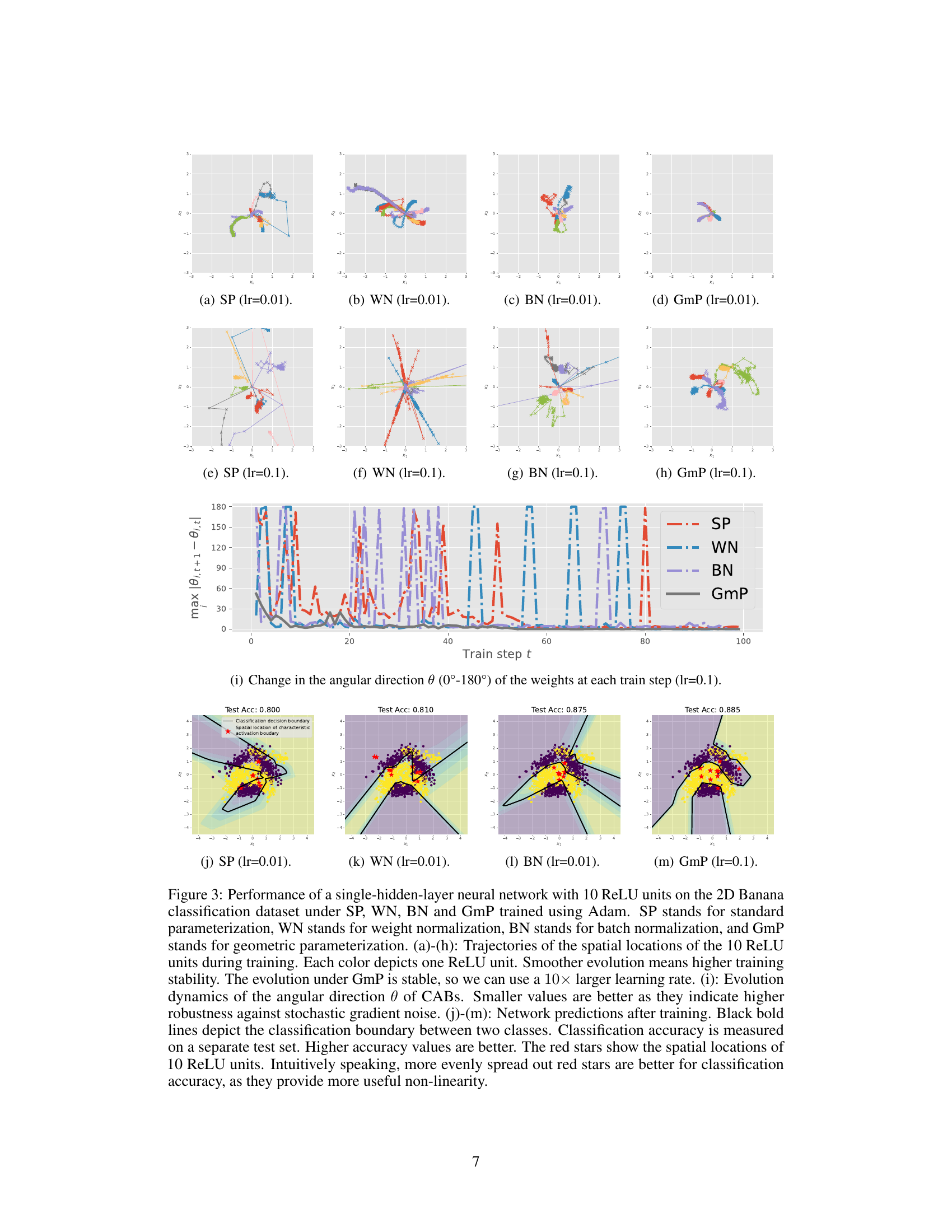
🔼 This figure shows the performance comparison of four different parameterization methods (SP, WN, BN, and GmP) on a 2D Banana classification task using a single-hidden-layer neural network with 10 ReLU units. Subfigures (a) through (h) illustrate the trajectories of the spatial locations of the ReLU units during training, highlighting the increased stability of GmP. Subfigure (i) visualizes the change in the angular direction of the characteristic activation boundaries (CABs), demonstrating GmP’s robustness to noise. Finally, subfigures (j) through (m) display the classification decision boundaries learned by each method, showcasing GmP’s superior performance and more even distribution of learned features.
read the caption
Figure 3: Performance of a single-hidden-layer neural network with 10 ReLU units on the 2D Banana classification dataset under SP, WN, BN and GmP trained using Adam. SP stands for standard parameterization, WN stands for weight normalization, BN stands for batch normalization, and GmP stands for geometric parameterization. (a)-(h): Trajectories of the spatial locations of the 10 ReLU units during training. Each color depicts one ReLU unit. Smoother evolution means higher training stability. The evolution under GmP is stable, so we can use a 10× larger learning rate. (i): Evolution dynamics of the angular direction θ of CABs. Smaller values are better as they indicate higher robustness against stochastic gradient noise. (j)-(m): Network predictions after training. Black bold lines depict the classification boundary between two classes. Classification accuracy is measured on a separate test set. Higher accuracy values are better. The red stars show the spatial locations of 10 ReLU units. Intuitively speaking, more evenly spread out red stars are better for classification accuracy, as they provide more useful non-linearity.

🔼 This figure shows the results of training a single-hidden-layer neural network with 10 ReLU units on the 2D Banana classification dataset using four different parameterization methods: Standard Parameterization (SP), Weight Normalization (WN), Batch Normalization (BN), and Geometric Parameterization (GmP). It compares the stability of the training process, the evolution of the characteristic activation boundaries (CABs), and the resulting classification accuracy. GmP shows significantly better stability and higher accuracy.
read the caption
Figure 3: Performance of a single-hidden-layer neural network with 10 ReLU units on the 2D Banana classification dataset under SP, WN, BN and GmP trained using Adam. SP stands for standard parameterization, WN stands for weight normalization, BN stands for batch normalization, and GmP stands for geometric parameterization. (a)-(h): Trajectories of the spatial locations of the 10 ReLU units during training. Each color depicts one ReLU unit. Smoother evolution means higher training stability. The evolution under GmP is stable, so we can use a 10× larger learning rate. (i): Evolution dynamics of the angular direction θ of CABs. Smaller values are better as they indicate higher robustness against stochastic gradient noise. (j)-(m): Network predictions after training. Black bold lines depict the classification boundary between two classes. Classification accuracy is measured on a separate test set. Higher accuracy values are better. The red stars show the spatial locations of 10 ReLU units. Intuitively speaking, more evenly spread out red stars are better for classification accuracy, as they provide more useful non-linearity.

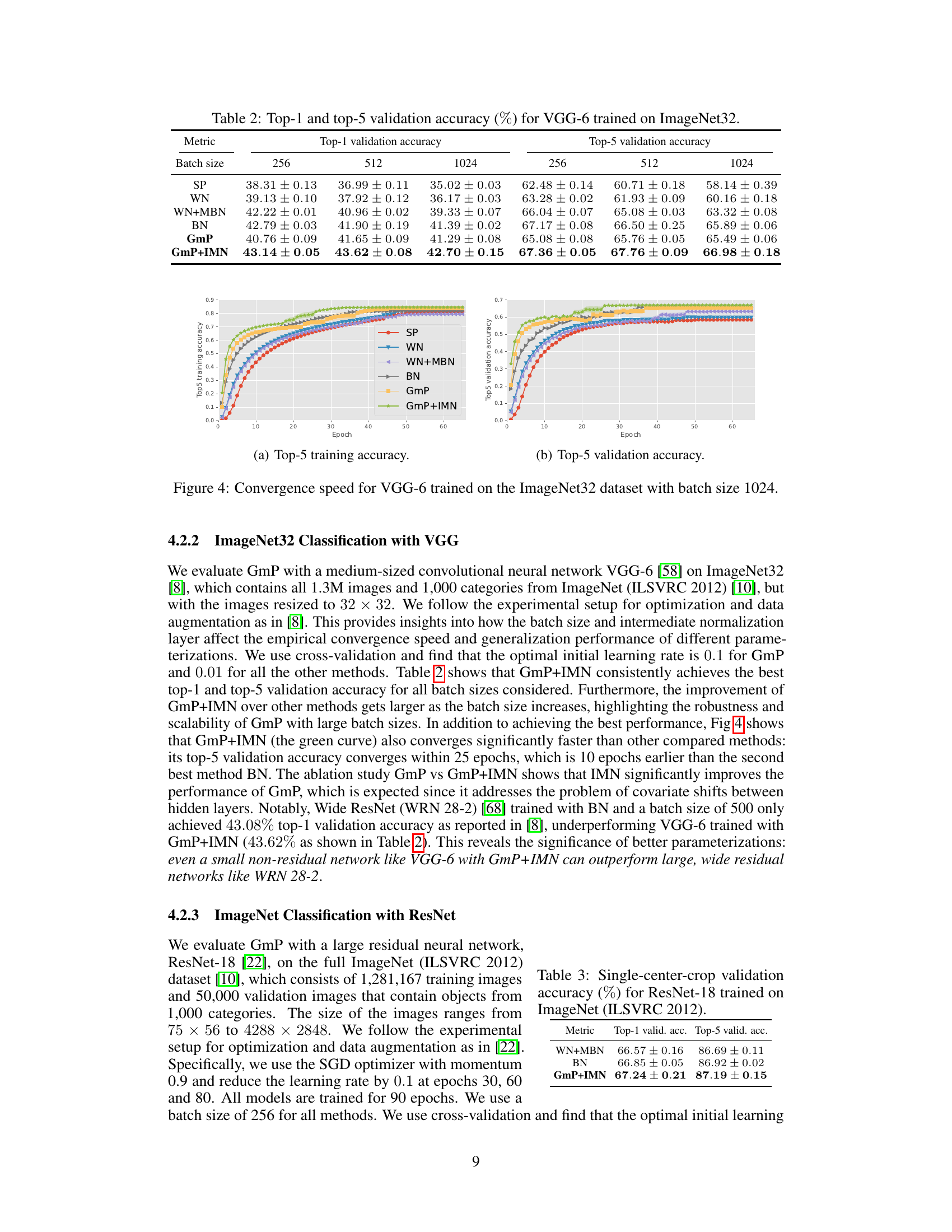
🔼 This figure shows the training and validation accuracy for VGG-6, a convolutional neural network, trained on the ImageNet32 dataset. Different parameterization methods (SP, WN, WN+MBN, BN, GmP, GmP+IMN) are compared, demonstrating that GmP+IMN achieves faster convergence with higher accuracy. The batch size is kept constant at 1024.
read the caption
Figure 4: Convergence speed for VGG-6 trained on the ImageNet32 dataset with batch size 1024.

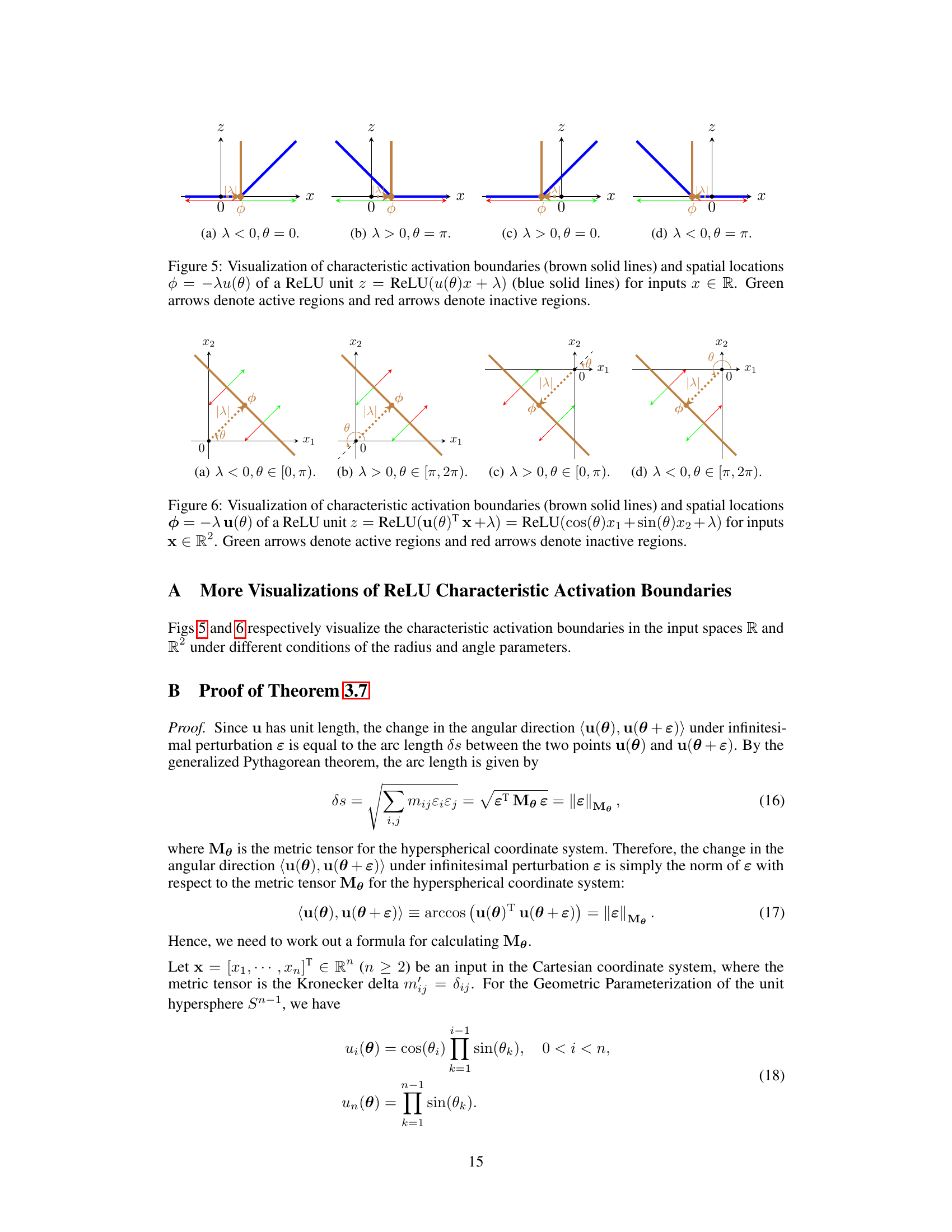
🔼 This figure visualizes the characteristic activation boundaries and spatial locations for a ReLU unit in one dimension. It illustrates how the boundary (represented by the brown line) and its location (blue line) change depending on different parameter settings (λ and θ). The active and inactive regions are also shown.
read the caption
Figure 5: Visualization of characteristic activation boundaries (brown solid lines) and spatial locations φ = −λα(θ) of a ReLU unit z = ReLU(u(θ)x + λ) (blue solid lines) for inputs x ∈ R. Green arrows denote active regions and red arrows denote inactive regions.

🔼 This figure shows the characteristic activation boundary (CAB) and its stability under different parameterizations. (a) illustrates a CAB as a line in 2D space separating active and inactive regions of a ReLU neuron. (b)-(e) demonstrate the effect of small perturbations on the CAB’s position for different parameterizations (SP, WN, BN, and GmP). The smaller the change in the CAB’s position after perturbation, the higher the stability of that parameterization. GmP shows the highest stability.
read the caption
Figure 1: (a) Characteristic activation boundary (CAB) B (brown solid line) and spatial location φ = −λu(θ) of a ReLU unit z = ReLU(u(θ)x + λ) = ReLU(cos(θ)x₁ + sin(θ)x₂ + λ) for inputs x ∈ R². The CAB forms a line in R², which acts as a boundary separating inputs into two regions. Green arrows denote the active region, and red arrows denote the inactive region. (b)-(e) Stability of the CAB of a ReLU unit in R² under small perturbations ε = δ₁ to the parameters. Solid lines denote characteristic activation boundaries B, and colored dotted lines connect the origin and spatial locations φ of B. Smaller changes between the perturbed and original boundaries imply higher stability. GmP is most stable against perturbations.
More on tables

🔼 This table presents the Top-1 and Top-5 validation accuracy results for a VGG-6 model trained on the ImageNet32 dataset. The results are broken down by different batch sizes (256, 512, and 1024) and different parameterization methods (SP, WN, WN+MBN, BN, GmP, and GmP+IMN). The table allows for comparison of the performance of different parameterization techniques under varying batch sizes, highlighting potential differences in training stability and generalization.
read the caption
Table 2: Top-1 and top-5 validation accuracy (%) for VGG-6 trained on ImageNet32.

🔼 This table presents the single-center-crop validation accuracy results for ResNet-18, a large residual neural network, trained on the full ImageNet dataset. The results are categorized by three different parameterization methods: WN+MBN, BN, and GmP+IMN, showing the top-1 and top-5 validation accuracy for each. The table highlights the superior performance of GmP+IMN, which demonstrates its effectiveness in large-scale residual network training.
read the caption
Table 3: Single-center-crop validation accuracy (%) for ResNet-18 trained on ImageNet (ILSVRC 2012).
Full paper#
