TL;DR#
Graph Neural Networks (GNNs) trained using self-supervised learning methods have shown great promise but are computationally expensive. This paper investigates the efficiency of these models by exploring the redundancy within their parameters. The researchers surprisingly found that a significant portion of parameters in these models are redundant and can be removed without affecting performance. This is true both at the neuron and layer levels.
To leverage this discovery, the authors propose a new framework called SLIDE (SLimming DE-correlation Fine-tuning). SLIDE first reduces the model size by removing redundant parameters. Then, it uses a de-correlation strategy during fine-tuning to further improve the performance. The experimental results show that SLIDE consistently outperforms traditional fine-tuning methods while requiring significantly fewer parameters, thereby improving the efficiency and reducing computational cost of GNNs.
Key Takeaways#
Why does it matter?#
This paper is crucial because it challenges the common assumption that all parameters in self-supervised graph neural networks (GNNs) are equally important. By demonstrating significant model redundancy, it opens avenues for creating more efficient and faster GNNs with fewer parameters, a critical need in the field. The proposed SLIDE framework offers a practical approach for achieving this and can influence future research in model optimization and pre-training techniques.
Visual Insights#

🔼 This figure illustrates three different methods for creating smaller variants of self-supervised pre-trained Graph Neural Networks (GNNs). The first method involves proportionally reducing the number of neurons in each layer. The second shows the original, full-sized GNN. The third method retains only the first two layers, while proportionally reducing the number of neurons in the second layer. These variations are used to investigate the impact of reduced model size on performance.
read the caption
Figure 1: Neuron dropout. To initialize a smaller variant of the self-supervised pre-trained GNNs, we select parameters from self-supervised GNNs in different ways. From left to right: randomly reduce the number of neurons in each layer proportionally, the original GNNs, retain only the first two layers while randomly reducing the number of neurons in the second layer proportionally.
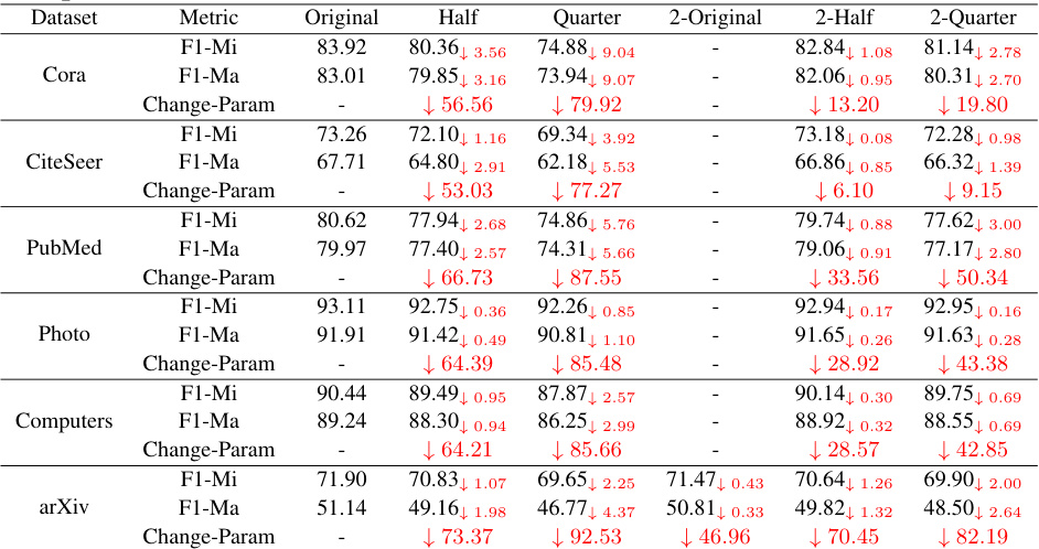
🔼 This table presents the performance of GraphMAE model on six datasets after applying different neuron removal methods. The methods vary the number of neurons retained, either proportionally across all layers or by removing layers entirely and altering the neurons in the remaining layers. The table shows the Micro-F1 and Macro-F1 scores for each method and dataset, along with the percentage change in the number of parameters compared to the original model. This illustrates the model’s redundancy by demonstrating how much performance is retained even with a significant reduction in parameters.
read the caption
Table 1: The performance of different neuron removal methods on six datasets with GraphMAE.
In-depth insights#
Redundancy in GNNs#
The concept of “Redundancy in GNNs” explores the unexpected observation that a significant portion of parameters within Graph Neural Networks (GNNs), particularly those trained via self-supervised learning, may be redundant without impacting performance. This redundancy suggests that substantial model compression is achievable. The paper investigates this phenomenon at both the neuron and layer levels, demonstrating that randomly removing a large percentage of parameters still results in high accuracy. This discovery has significant implications for model efficiency and resource usage. The observed redundancy necessitates a reevaluation of the GNN training paradigm, suggesting the need for methods that explicitly address and leverage this inherent characteristic for improved resource utilization and potentially even enhanced performance. Further research should focus on developing techniques for strategically identifying and removing redundant parameters, optimizing model architectures, and refining the training process to take advantage of this property.
SLIDE Framework#
The SLIDE framework, a novel graph pre-training and fine-tuning paradigm, addresses the limitations of existing methods by directly tackling the redundancy inherent in graph self-supervised learning models. SLIDE’s core innovation lies in its two-pronged approach: model slimming and de-correlation fine-tuning. By strategically reducing the number of neurons and layers (slimming), SLIDE efficiently removes redundant model parameters without significantly impacting performance, improving computational efficiency. Furthermore, SLIDE incorporates a de-correlation strategy during fine-tuning to minimize the redundancy between learned feature representations. This enhances the informativeness of the remaining parameters, leading to improved downstream task performance. The framework’s effectiveness is empirically validated across various benchmarks, demonstrating improvements over conventional fine-tuning approaches with fewer parameters. Overall, SLIDE provides a powerful and efficient pathway for leveraging the benefits of graph self-supervised learning while mitigating the challenges associated with model redundancy and computational cost.
Ablation Study#
An ablation study systematically removes components of a model to assess their individual contribution. In the context of a graph self-supervised learning model, this might involve removing neurons, layers, or specific augmentation techniques. The goal is to understand which parts are essential for good performance and which are redundant. By selectively disabling model components and observing the impact on downstream tasks (e.g., node classification), researchers can identify crucial elements and potentially simplify the model for better efficiency without sacrificing accuracy. This also helps in understanding the model’s behavior, revealing which elements are more critical for learning specific features or handling certain types of graph structures. The results from such a study provide valuable insights for model optimization and architectural design, guiding the development of more effective and streamlined graph self-supervised learning methods. A well-designed ablation study is crucial for demonstrating the contributions of individual components and validating the overall model architecture. Finally, it allows for a deeper understanding of why a model works, potentially uncovering insights into the underlying mechanisms of graph representation learning.
Parameter Analysis#
A parameter analysis in a deep learning context, especially within the realm of graph neural networks (GNNs), is crucial for understanding model efficiency and performance. It involves investigating the impact of the number of parameters (weights and biases) on downstream task accuracy and computational cost. A key insight often uncovered is the presence of redundancy, where a significant portion of the parameters might contribute minimally to performance. This suggests that models could be effectively ‘slimmed down’ without sacrificing accuracy, leading to faster training and inference times. The analysis should delve into the distribution of parameter importance, potentially employing techniques like pruning or identifying less critical layers. The analysis should also consider the interplay between parameter reduction and the choice of optimization strategies. Different optimization algorithms might exhibit varying sensitivities to parameter reductions, so an effective analysis should account for this interplay. Ultimately, the goal is to uncover optimal parameter configurations for maximal efficiency without compromising accuracy, offering valuable insights into resource-efficient model design and deployment.
Future Work#
Future research directions stemming from this paper could explore several promising avenues. Extending the SLIDE framework to other GNN architectures and downstream tasks beyond node classification is crucial to establish its generalizability. A deeper investigation into the theoretical underpinnings of model redundancy in graph self-supervised learning is needed, potentially leveraging tools from information theory or statistical mechanics. Developing more sophisticated de-correlation techniques that go beyond the Frobenius norm, perhaps incorporating advanced regularization methods or adversarial training, could significantly boost performance. Furthermore, examining the impact of different graph augmentation strategies on model redundancy and the effectiveness of SLIDE would be valuable. Finally, a comprehensive empirical comparison against other parameter-efficient fine-tuning methods, such as LoRA or Adapter Tuning, is warranted to fully showcase the advantages of this approach. These advancements would solidify the practical impact and theoretical understanding of model redundancy in graph neural networks.
More visual insights#
More on figures

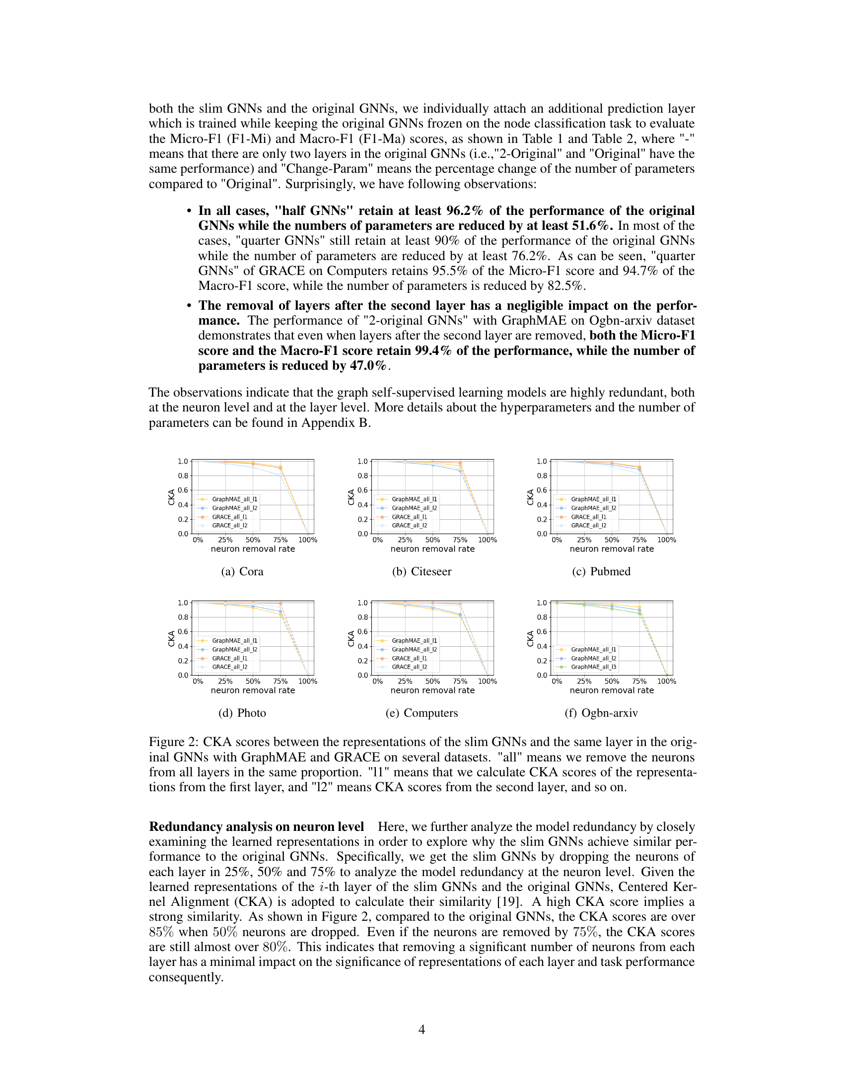
🔼 This figure displays the centered kernel alignment (CKA) scores, a measure of similarity between representations, for slim GNNs (Graph Neural Networks with reduced neurons) and their corresponding layers in the original GNNs. Different datasets (Cora, Citeseer, Pubmed, Photo, Computers, and Ogbn-arxiv) are shown, each with CKA scores calculated for the first, second, and potentially third layers of the model. The neuron removal rate (x-axis) indicates the percentage of neurons randomly removed from each layer. The results demonstrate the impact of neuron reduction on the similarity of representations between the slim GNNs and their full-sized counterparts, showing a remarkable degree of redundancy within the models.
read the caption
Figure 2: CKA scores between the representations of the slim GNNs and the same layer in the original GNNs with GraphMAE and GRACE on several datasets. 'all' means we remove the neurons from all layers in the same proportion. '11' means that we calculate CKA scores of the representations from the first layer, and '12' means CKA scores from the second layer, and so on.

🔼 This figure visualizes the redundancy analysis on the layer level using Centered Kernel Alignment (CKA) scores. It shows the CKA scores between the representations of each layer and its adjacent layer in the original Graph Neural Networks (GNNs) for two different graph self-supervised learning models, GraphMAE and GRACE. High CKA scores (close to 1) indicate high similarity between representations of adjacent layers, suggesting redundancy in the model’s design. The low CKA score between the original features and the representation of the first layer is also shown.
read the caption
Figure 3: CKA scores between the representations of each layer and its adjacent layer of the original GNNs for GraphMAE and GRACE on several datasets.
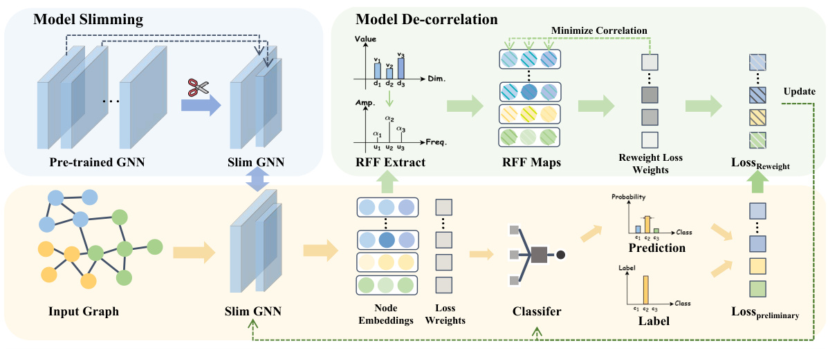
🔼 The figure illustrates the overall framework of the SLIDE (SLIm DE-correlation Fine-tuning) method. It is divided into two main parts: model slimming and model de-correlation. The model slimming part takes a pre-trained GNN and reduces it to a slimmer version by removing redundant neurons. The model de-correlation part takes the output embeddings from the slim GNN, applies Random Fourier Features (RFF) to extract features, uses RFF maps to minimize the correlation between the features, and finally uses reweighted loss to update the weights and achieve better classification performance. The prediction and loss computation are shown in the bottom part of the figure.
read the caption
Figure 4: The overall framework of SLIDE.

🔼 This figure presents the ablation study results on the impact of model de-correlation in SLIDE. It shows the performance of SLIDE with and without de-correlation on six benchmark datasets (Cora, Citeseer, Pubmed, Photo, Computers, Ogbn-arxiv) across three pre-training frameworks (GraphMAE, GRACE, MaskGAE). The results are presented separately for Micro-F1 and Macro-F1 scores. The results demonstrate that incorporating the de-correlation module significantly improves the performance of SLIDE. The Ogbn-arxiv results with GRACE are missing due to memory limitations.
read the caption
Figure 5: Ablation studies of model de-correlation on six benchmark datasets and three pre-training frameworks. 'w/o de' means that we fine-tune the slim GNNs without model de-correlation methods. 'Mi' means Micro-F1 scores and 'Ma' means Macro-F1 scores. The results of Ogbn-arxiv with GRACE are unseen because of 'out of memory'.

🔼 This figure compares the number of parameters in the original model (full fine-tuning) versus the slimmed model (SLIDE) for GraphMAE and GRACE on several datasets. It visually demonstrates the significant reduction in parameters achieved by SLIDE without substantial performance loss, as reported in the paper.
read the caption
Figure 6: The number of parameters on several datasets with GraphMAE and GRACE.
More on tables
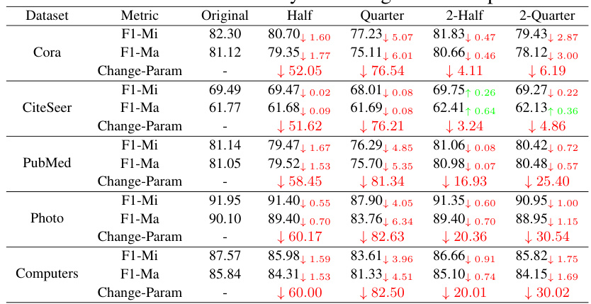
🔼 This table presents the results of experiments evaluating the performance of GraphMAE models after removing different proportions of neurons using various methods. The performance is measured using Micro-F1 (F1-Mi) and Macro-F1 (F1-Ma) scores across six datasets. The ‘Change-Param’ column indicates the percentage change in the number of parameters compared to the original model.
read the caption
Table 1: The performance of different neuron removal methods on six datasets with GraphMAE.

🔼 This table presents the results of node classification experiments using the GraphMAE model. It compares the performance of three different fine-tuning methods (Linear Probing, Full Fine-tuning, and SLIDE) across six benchmark datasets. The metrics reported are Micro-F1 and Macro-F1 scores, along with the percentage change in the number of parameters compared to the original model. It shows the performance of the model on the node classification task after the parameters are removed by different methods.
read the caption
Table 3: Node classification accuracy (%±σ) on six benchmark datasets with GraphMAE.
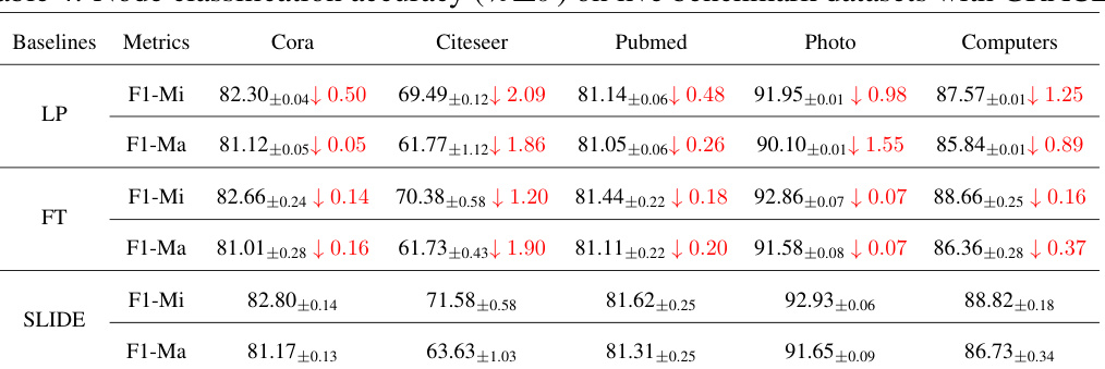
🔼 This table presents the performance of different node classification methods on six benchmark datasets using the GraphMAE framework. It compares three approaches: Linear Probing (LP), Full Fine-tuning (FT), and the proposed SLIDE method. The results are reported as accuracy with standard deviation, showing the Micro-F1 and Macro-F1 scores for each method and dataset. The ‘Change-Param’ column indicates the percentage change in the number of parameters compared to the original model. The table highlights the effectiveness of SLIDE in achieving comparable performance to full fine-tuning while using fewer parameters.
read the caption
Table 3: Node classification accuracy (%±σ) on six benchmark datasets with GraphMAE.

🔼 This table presents the performance of different node classification methods (Linear Probing, Full Fine-tuning, and SLIDE) using the GraphMAE framework on six benchmark datasets. The results are reported as accuracy with standard deviation, showing the impact of the neuron removal methods on classification performance. The ‘Change-Param’ column indicates the percentage change in the number of parameters compared to the original model. The table highlights the model redundancy in GraphMAE, where even with significant parameter reduction, the performance remains relatively high.
read the caption
Table 3: Node classification accuracy (%±σ) on six benchmark datasets with GraphMAE.

🔼 This table presents the performance of the MaskGAE model on three datasets (Cora, CiteSeer, PubMed) after removing neurons using different methods. It shows the Area Under the Curve (AUC) and Average Precision (AP) scores for link prediction. The ‘Change-Param’ row indicates the percentage of parameters removed in the ‘Half’ and ‘Quarter’ GNN models compared to the original GNNs.
read the caption
Table 6: The performance of different neuron removal methods on three datasets with MaskGAE on link prediction tasks.

🔼 This table presents the results of experiments evaluating the performance of GraphMAE models on four graph classification datasets after removing different proportions of neurons. The table shows the accuracy (ACC) achieved on each dataset after removing neurons at the neuron level (half, quarter) and layer level (2-original, 2-half, 2-quarter), and compares those accuracies to a model with no neuron removal (Original). The ‘Change-Param’ column shows the percentage of parameters removed in each slimmed model relative to the original model. The results illustrate the level of redundancy in the GraphMAE model.
read the caption
Table 7: The performance of different neuron removal methods on four datasets with GraphMAE on graph classification tasks.

🔼 This table shows the number of parameters in GNN and Linear layers for different datasets (Cora, CiteSeer, PubMed, Photo, Computers, arXiv) using GraphMAE. It breaks down the parameter counts for the original model and variations created by removing neurons using different methods (Half, Quarter, 2-Original, 2-Half, 2-Quarter). This allows for a comparison of parameter reduction strategies and their impact on the model’s size.
read the caption
Table 8: More details about paramters with different neuron removal methods for GraphMAE, where the parameters in GNN is not fine-tunable while the parameters in Linear is fine-tunable.
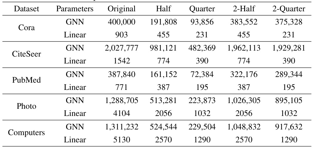
🔼 This table details the number of parameters (GNN and Linear) in the GraphMAE model before and after applying different neuron removal methods. It shows the original number of parameters, and then the number remaining after randomly removing 50% (Half), 75% (Quarter), 50% in the second layer (2-Half), and 75% in the second layer (2-Quarter) of the neurons. This breakdown helps illustrate the model’s redundancy by showing that a significant portion of parameters can be removed without substantial performance loss. The ‘Linear’ parameters refer to the classifier layer which is fine-tuned, while the ‘GNN’ parameters represent the pre-trained graph neural network.
read the caption
Table 8: More details about paramters with different neuron removal methods for GraphMAE, where the parameters in GNN is not fine-tunable while the parameters in Linear is fine-tunable.

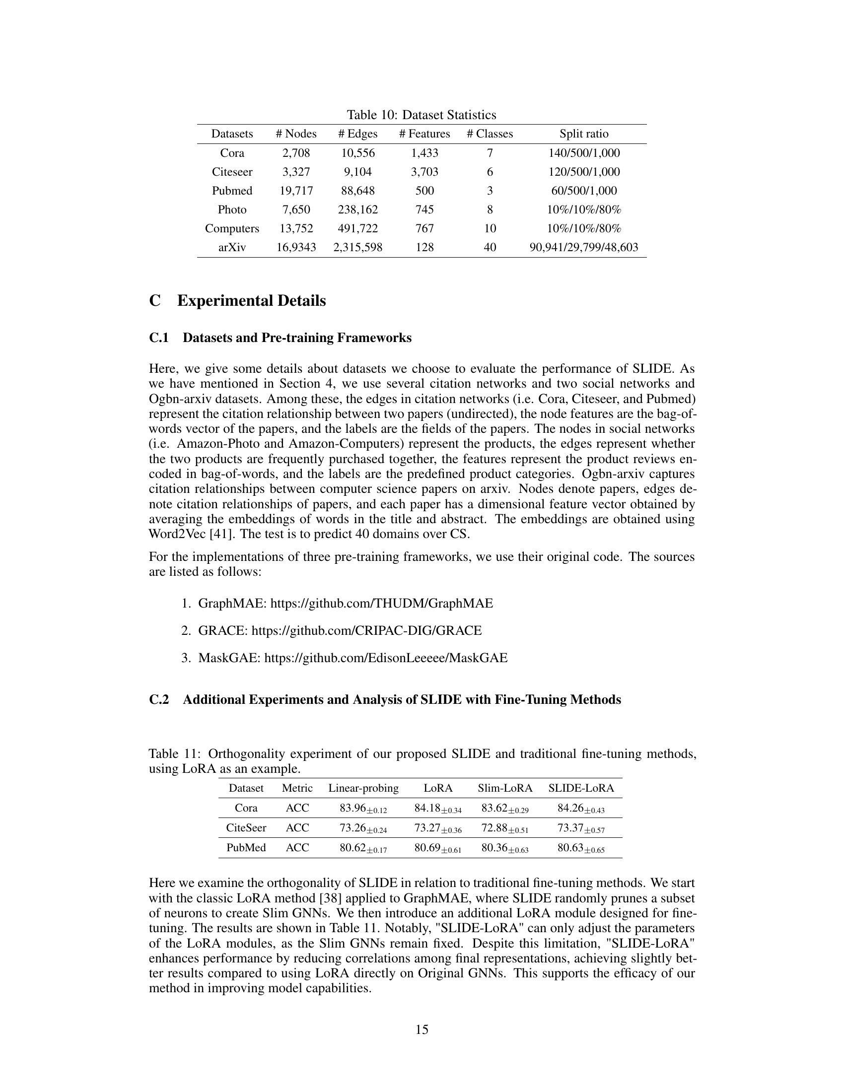
🔼 This table presents the statistics of the six benchmark datasets used in the paper’s experiments. For each dataset, it shows the number of nodes, edges, features, classes, and the split ratio for training, validation, and testing.
read the caption
Table 10: Dataset Statistics

🔼 This table presents the results of an experiment designed to show the orthogonality of the proposed SLIDE method with respect to traditional fine-tuning methods. The experiment uses the LoRA (Low-Rank Adaptation) method as a representative example of fine-tuning techniques. It compares the performance of linear probing, LoRA, Slim-LoRA (LoRA applied to a slimmed GNN), and SLIDE-LoRA (SLIDE combined with LoRA) on three datasets (Cora, CiteSeer, PubMed). The metric used is accuracy (ACC). The results demonstrate that SLIDE can be effectively combined with other fine-tuning methods to improve model performance.
read the caption
Table 11: Orthogonality experiment of our proposed SLIDE and traditional fine-tuning methods, using LoRA as an example.
Full paper#
