Great Minds Think Alike: The Universal Convergence Trend of Input Salience

7PORYhql4V

Yipei Wang et el.

TL;DR
#

Deep learning models, despite their complexity, exhibit unexpected regularities. This paper investigates the distribution of optimized deep neural networks (DNNs) trained with stochastic algorithms. A key challenge in deep learning is the inherent stochasticity of training, leading to a distribution of different optimized models, and understanding this distribution’s properties is crucial.

The researchers focus on input salience maps which represent the sensitivity of the model’s prediction to different input features. Their main finding is that as model capacity increases, the input salience of optimized DNNs converges towards a shared mean. This convergence trend is independent of the specific architecture of the model and consistently occurs across various model types. They introduced a semi-parametric approach for modeling this convergence, which helps explain several previously unclear phenomena, such as the efficacy of deep ensemble methods.

Key Takeaways
#

Why does it matter?
#

This paper is crucial because it significantly advances our understanding of deep neural network (DNN) behavior, particularly concerning the distribution of optimized models. It offers valuable insights for improving DNN performance, enhancing adversarial robustness, and better understanding deep ensemble methods. By revealing the hidden similarities in input salience, the research opens exciting avenues for future investigations in various areas of deep learning.

Visual Insights
#

🔼 This figure provides a synthetic illustration to visualize the hypothesis of the paper regarding the distribution of directional gradients (input salience) of stochastically optimized models. Panel (a) shows a scenario where distributions for different model families are independent, while panel (b) shows the converging trend hypothesized in the paper as model capacity increases. Different colors represent different model families, and each point represents a different optimized model.
read the caption
Figure 1: A synthetic illustration of the distribution of the directional gradients of stochastically optimized models of the same input data. The subfigures demonstrate (a) an intuitive, stochastic scenario, where the distributions of different model families are not closely dependent, and (b) the converging distribution trend introduced by our hypothesis. Different colors represent different model families, and points represent different optimized models.

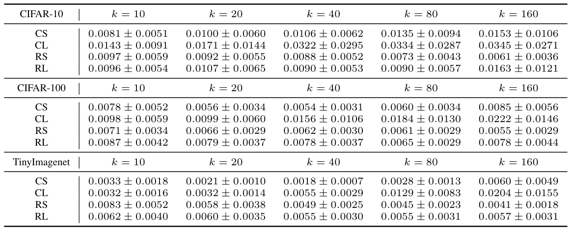
🔼 This table presents the average Wasserstein distances between the salience distributions of different models within the same family, showing how the distance changes with model capacity (k) and architecture. The baseline distance is 2, reflecting the range of cosine similarity values. The table shows that deeper models (CL vs CS, RL vs RS) tend to have greater distances between their salience distributions, possibly due to increased training difficulty.
read the caption
Table 1: The average Wasserstein distance E_{f(1),f(2)∈F(k)}WD(S(f(1)),S(f(2)) ) with the standard deivation for all model families {CS,CL,RS,RL}×{10,20,40,80,160} over CIFAR-10/100 and TinyImagenet datasets. Note that here the baseline should be 2 since the cosine similarity lies in [-1,1]. It is observed that deeper models usually have larger distances (CS vs. CL, RS vs. RL). We deduce that this is because of the training for deeper models is more difficult.

In-depth insights
#

DNN Salience Trends
#

Analyzing Deep Neural Network (DNN) salience trends reveals crucial insights into model behavior and generalization. The distribution of salience maps across different, stochastically trained DNNs, even with varying capacities, demonstrates a surprising convergence. Larger models tend to exhibit more aligned salience patterns, indicating a shared underlying mechanism for interpreting input features. This convergence has significant implications for deep learning, including improving our understanding of adversarial robustness and explaining the effectiveness of ensemble methods. The alignment in salience direction suggests a universal trend, where different models prioritize similar input regions. This pattern highlights the potential for improved model interpretability and explainability by focusing on shared features across multiple model outputs. Further research investigating these convergence trends is crucial for advancing our understanding of DNNs and developing more reliable and robust AI systems.

Convergence Analysis
#

A convergence analysis in a deep learning context would typically involve examining how the model’s parameters evolve during training and whether they approach a stable state. This could encompass investigating the behavior of loss functions over epochs, evaluating the change in model accuracy on training and validation datasets, and analyzing the gradients of the loss function to understand the optimization dynamics. Key aspects to consider would be the rate of convergence, whether the model converges to a global or local minimum, and the impact of hyperparameters on the convergence process. The analysis might also include visualizing the parameter space or using mathematical techniques like examining eigenvalue distributions to gain insights into the stability and convergence behavior. For stochastic gradient descent (SGD), the analysis would need to address the inherent randomness and explore the convergence in expectation or probability. The ultimate goal of such an analysis is to gain a deeper understanding of how models learn, pinpoint potential problems hindering optimal performance (e.g., poor generalization), and improve training strategies for faster and more stable learning.

Saw Dist. Modeling
#

The heading ‘Saw Dist. Modeling’ suggests a methodological approach within the research paper that utilizes the Sawtooth distribution (or a variation thereof) for modeling a specific phenomenon. The Sawtooth distribution, known for its unique shape with a concentration of probability near its mean and then a gradual tapering off, is likely employed because it might effectively capture the distribution’s behavior. This is especially useful if the observed data exhibits this characteristic concentration and tapering. The choice of Sawtooth distribution reflects a considered decision about the appropriate statistical model which could be justified by the nature of the data or insights from exploratory data analysis. Within the paper, the use of this model will likely involve parameter estimation and model fitting techniques. A key strength of this approach could be its ability to describe the underlying trend in the data more accurately compared to simpler models, whilst also enabling deeper interpretation of the model parameters in the context of the research. However, limitations might arise from assumptions underlying the Sawtooth distribution. The model’s success critically depends on the appropriateness of these assumptions to the underlying data-generating process. Further validation and justification are required within the paper.

Black-box Attack
#

The research paper explores black-box attacks in the context of deep neural networks (DNNs), focusing on the implications of the universal convergence trend of input salience. The core idea is that the input salience, which essentially represents the sensitivity of a DNN’s output to changes in its input, exhibits surprising similarities across different, stochastically trained models. This similarity is particularly pronounced as model capacity increases, leading to higher resemblance in their mean saliency direction. This has significant implications for black-box attacks, where the internal structure of the target model is unknown and the attacker must rely on readily observable information (like input gradients) to craft adversarial examples. The high degree of salience similarity means that an attack crafted against one model will often effectively transfer to other models, especially larger ones. This transferability is not merely an empirical phenomenon but arises naturally from the convergence of saliency distributions; hence, attacking via the estimated mean salience direction can often be even more effective than targeting individual models. This observation also sheds light on the effectiveness of deep ensembles, as these effectively approximate the mean salience direction using multiple models. In summary, the work provides a theoretical explanation for the practical success of deep ensembles and a novel perspective on the vulnerability of large DNNs to black-box attacks.

Deep Ensemble
#

Deep ensembles, which involve training multiple neural networks independently and combining their predictions, offer several advantages. The primary benefit is improved prediction accuracy, often exceeding that of a single, larger model. This improvement arises from the ensemble’s ability to reduce variance and capture diverse aspects of the underlying data distribution. Robustness is another key advantage, as ensembles often show greater resistance to noisy or adversarial inputs than individual models. This stems from the averaging effect, where outliers from individual models are mitigated. However, deep ensembles also present challenges. Computational cost is significantly increased due to the need for training multiple models. Interpretability is reduced, making it harder to understand the decision-making process of the ensemble. Furthermore, the optimal number of ensemble members and their individual architectures require careful consideration and tuning. Understanding the underlying reasons for the success of deep ensembles remains a subject of ongoing research. Future work should explore strategies to reduce the computational burden while retaining the ensemble’s benefits.

More visual insights
#

More on figures

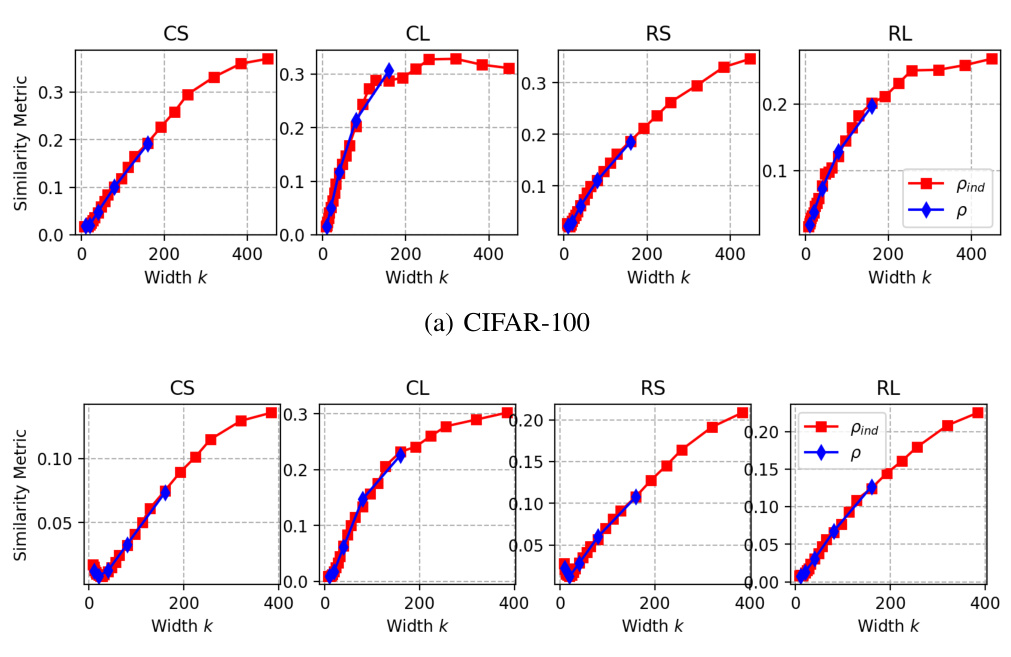
🔼 This figure shows the individual similarity between input salience of two models f(1) and f(2) which belong to model families with different capacities (k1 and k2). The similarity is measured using cosine similarity of input gradients over the test dataset. The figure presents results for CIFAR-10 and CIFAR-100 datasets, with both CNN and ResNet model architectures.
read the caption
Figure 2: The individual similarity pind(f(1), f(2)) = Ex∈x[CosSim(∇æ f(1)(x), ∇æ f(2)(x))], where f(1) ∈ F(k1), f(2) ∈ F(k2). CIFAR-10/100 and CNN & ResNets are tested here.

🔼 This figure displays the individual similarity between input salience of two models with varying capacities (k1 and k2). The similarity is measured using cosine similarity of input gradients across the test set. Results are shown for CIFAR-10 and CIFAR-100 datasets, using both CNN and ResNet model architectures.
read the caption
Figure 2: The individual similarity pind(f(1), f(2)) = Ex∈x[CosSim(∇æ f(1)(x), ∇æ f(2)(x))], where f(1) ∈ F(k1), f(2) ∈ F(k2). CIFAR-10/100 and CNN & ResNets are tested here.

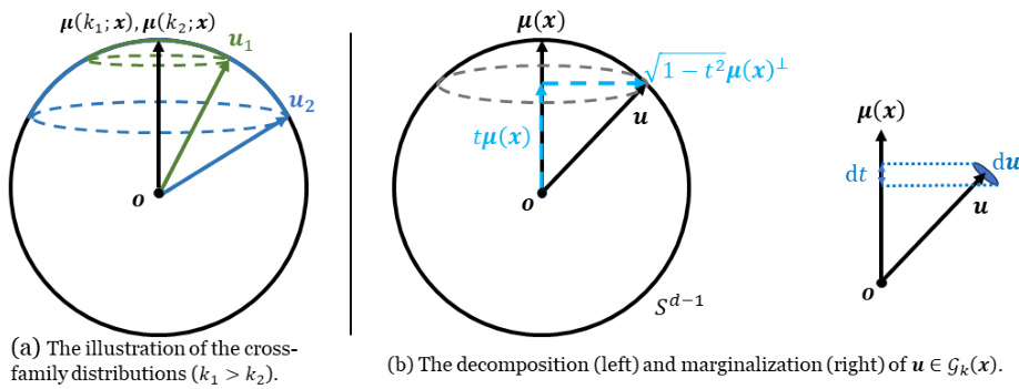
🔼 This figure provides a visualization of the two hypotheses (H1 and H2) proposed in the paper regarding the distribution of input salience in deep neural networks (DNNs). Panel (a) shows how the distributions of input gradient directions for different model families (colors) converge towards a common mean direction as model capacity (k) increases. This illustrates both H1 (increasing capacity leads to smaller spherical variance) and H2 (mean directions align across families). Panel (b) breaks down the mathematical representation of the process. The left side shows how a gradient vector (u) can be decomposed into a component along the mean direction (tμ(x)) and a component orthogonal to it (√1−t²μ(x)⊥). The right side illustrates the marginalization process focusing on the distribution of t, the projection of u onto the mean direction.
read the caption
Figure 4: (a) presents an illustration of H1 and H2. Blue and green caps represent u₁ ∈ Gk₁(x) (green) and u₂ ∈ Gk₂(x) (blue) regions 2. H1: larger ks lead to smaller spherical variances; H2: the mean directions are extremely similar. (b) illustrates (left) the decomposition of u to the mean direction and the orthogonal direction; and (right) the marginalization of the distribution from u to t.

🔼 This figure provides a synthetic visualization to illustrate the hypothesis of the paper regarding the distribution of input salience maps of stochastically trained models. (a) shows a random distribution where model families (represented by colors) are independent. (b) illustrates the hypothesized convergent trend where model families align as capacity increases, showing a shared population mean direction.
read the caption
Figure 1: A synthetic illustration of the distribution of the directional gradients of stochastically optimized models of the same input data. The subfigures demonstrate (a) an intuitive, stochastic scenario, where the distributions of different model families are not closely dependent, and (b) the converging distribution trend introduced by our hypothesis. Different colors represent different model families, and points represent different optimized models.

🔼 This figure shows the individual similarity between input salience maps of two stochastically optimized models with varying capacities (k1 and k2). The similarity is measured using the cosine similarity of the input gradients. Experiments are performed on CIFAR-10 and CIFAR-100 datasets, using both CNN and ResNet model architectures. The heatmaps illustrate how similarity changes depending on model capacity.
read the caption
Figure 2: The individual similarity pind(f(1), f(2)) = Ex∈x[CosSim(∇æ f(1)(x), ∇æ f(2)(x))], where f(1) ∈ F(k1), f(2) ∈ F(k2). CIFAR-10/100 and CNN & ResNets are tested here.

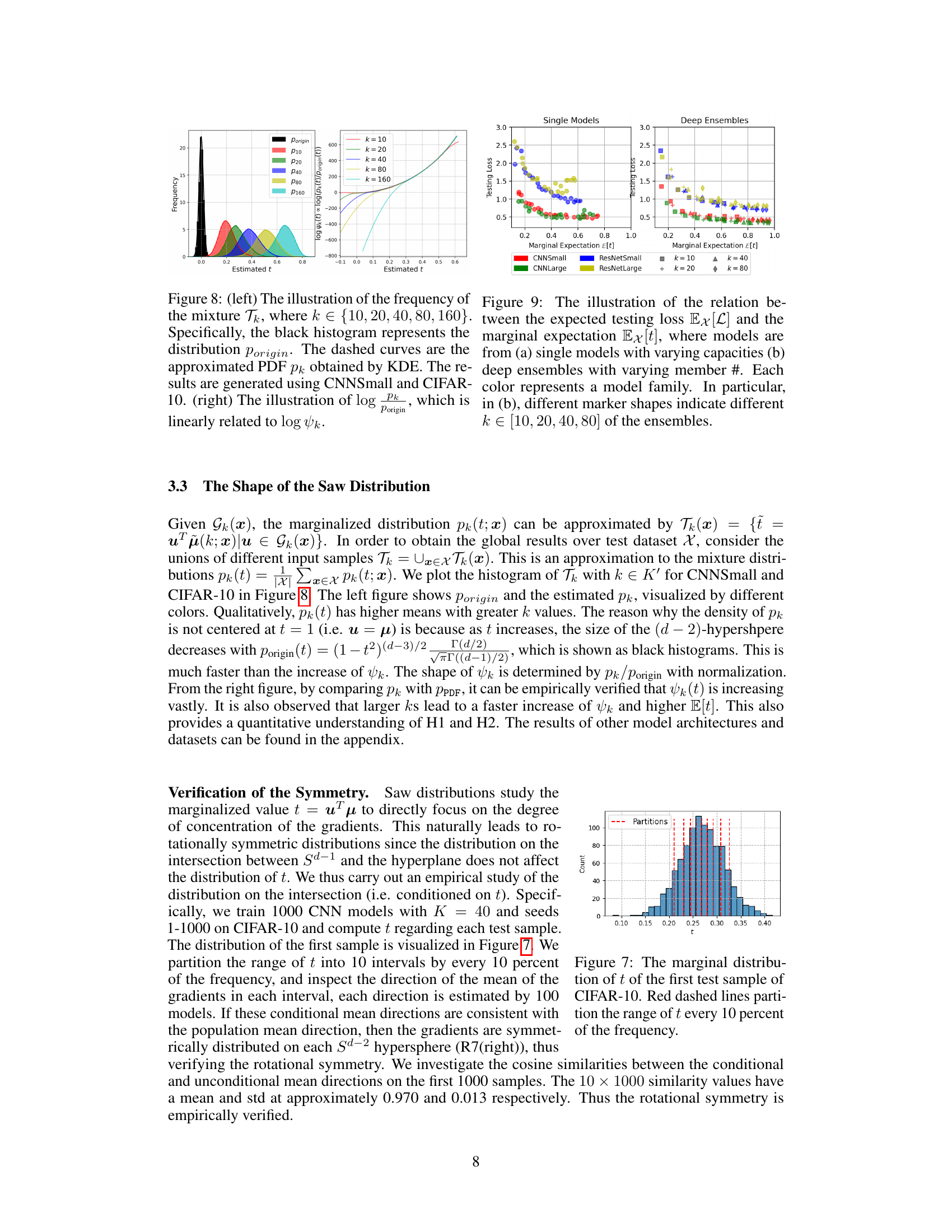
🔼 This figure shows the empirical results that support Hypothesis I and Hypothesis II. The left panel shows the estimated probability density functions (PDFs) of the marginal distribution of the cosine similarity between input saliency maps (denoted as t) for different model widths (k). The black histogram represents the PDF of uniformly distributed data on a hypersphere. The colored curves represent the estimated PDFs of t for varying k, which are approximated using kernel density estimation (KDE). The right panel shows the relationship between log(pk) and log(ψk), which demonstrates the relationship between the estimated PDF of t and the shape function of the Saw distribution.
read the caption
Figure 8: (left) The illustration of the frequency of the mixture Tk, where k ∈ {10, 20, 40, 80, 160}. Specifically, the black histogram represents the distribution Porigin. The dashed curves are the approximated PDF pk obtained by KDE. The results are generated using CNNSmall and CIFAR-10. (right) The illustration of log pk, which is linearly related to log ψk.

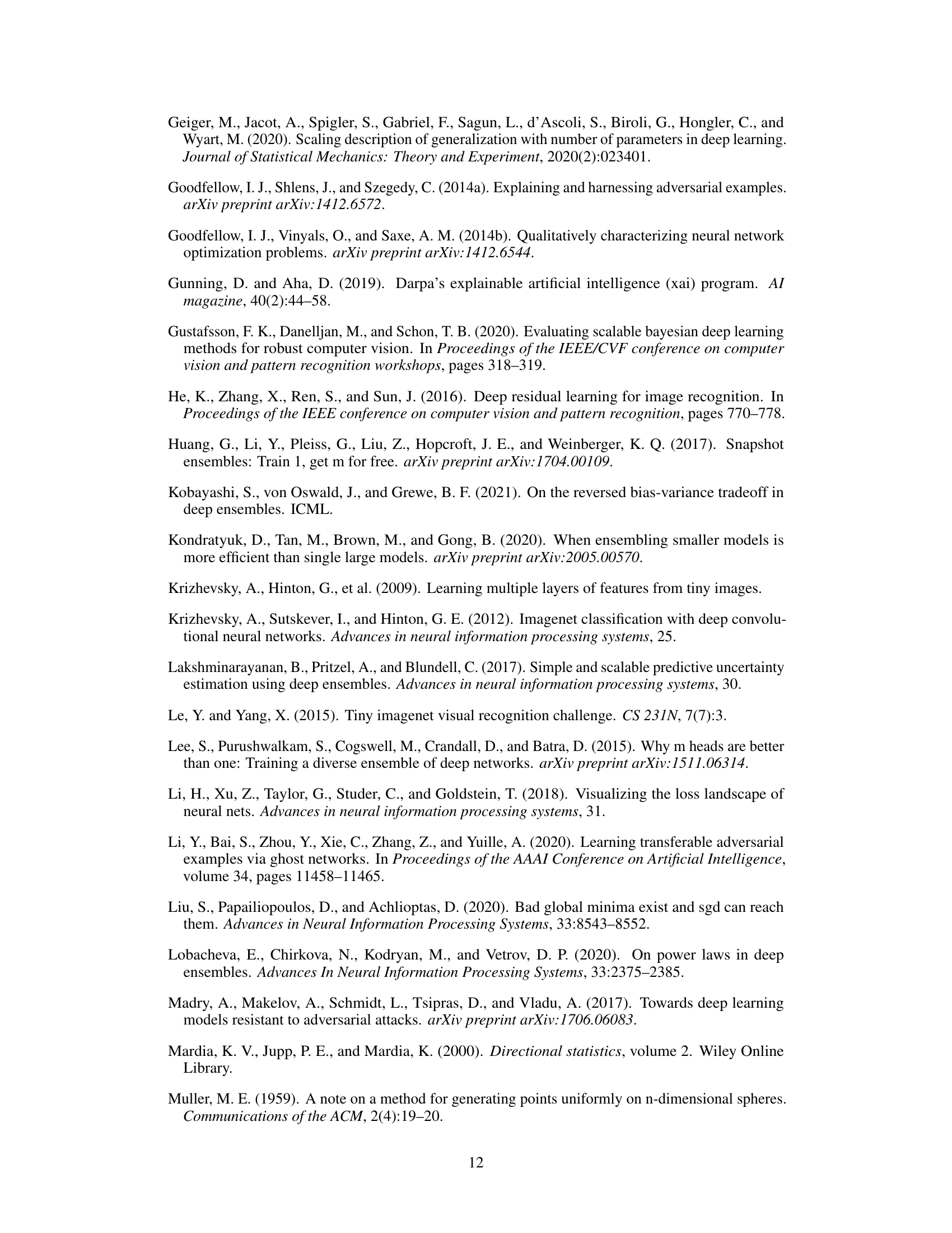
🔼 This figure shows the marginal distribution of t, where t is the cosine similarity between the gradient direction of a model and the mean gradient direction. The distribution is shown for the first test sample of the CIFAR-10 dataset. Red dashed lines divide the distribution into deciles (10% increments) to show the density in different regions of the distribution.
read the caption
Figure 7: The marginal distribution of t of the first test sample of CIFAR-10. Red dashed lines partition the range of t every 10 percent of the frequency.

🔼 This figure shows the individual similarity between input salience of two models, f(1) and f(2), with varying capacities (k1 and k2). The similarity is measured using the cosine similarity of their input gradients across the entire test set. The results are shown for CIFAR-10 and CIFAR-100 datasets, using both CNN and ResNet architectures. The figure aims to visually demonstrate the increasing trend of similarity as model capacities (k1 and k2) increase.
read the caption
Figure 2: The individual similarity pind(f(1), f(2)) = Ex∈x[CosSim(∇æ f(1)(x), ∇æ f(2)(x))], where f(1) ∈ F(k1), f(2) ∈ F(k2). CIFAR-10/100 and CNN & ResNets are tested here.

🔼 This figure compares the effectiveness of three different black-box attack strategies. The first uses the gradients from the largest model in the same model family as the target model (red). The second uses the gradients from a model with the same capacity as the target model (green). The third utilizes the mean gradient direction across all model families (blue). The results are presented as a prediction decay ratio (α) plotted against the width of the target model. This helps visualize how effectively each attack strategy influences the performance of the target model.
read the caption
Figure 11: The comparison between the single-model attack from the largest model (red), the single-model attack from the very same capacity (green) and the attack by the mean direction (blue).

🔼 This figure illustrates the difference between a random distribution of model gradients (a) and a converging distribution (b), which is a key hypothesis of the paper. The converging trend shows that models with increasing capacity tend to align in terms of their input salience, even if trained stochastically.
read the caption
Figure 1: A synthetic illustration of the distribution of the directional gradients of stochastically optimized models of the same input data. The subfigures demonstrate (a) an intuitive, stochastic scenario, where the distributions of different model families are not closely dependent, and (b) the converging distribution trend introduced by our hypothesis. Different colors represent different model families, and points represent different optimized models.

🔼 This figure shows the individual similarity between input salience of two models f(1) and f(2) from different families F(k1) and F(k2) with varying capacities k1 and k2. The similarity is measured using cosine similarity of input gradients. The experiments were conducted on CIFAR-10 and CIFAR-100 datasets using CNN and ResNet model architectures.
read the caption
Figure 2: The individual similarity pind(f(1), f(2)) = Ex∈x[CosSim(∇æ f(1)(x), ∇æ f(2)(x))], where f(1) ∈ F(k1), f(2) ∈ F(k2). CIFAR-10/100 and CNN & ResNets are tested here.

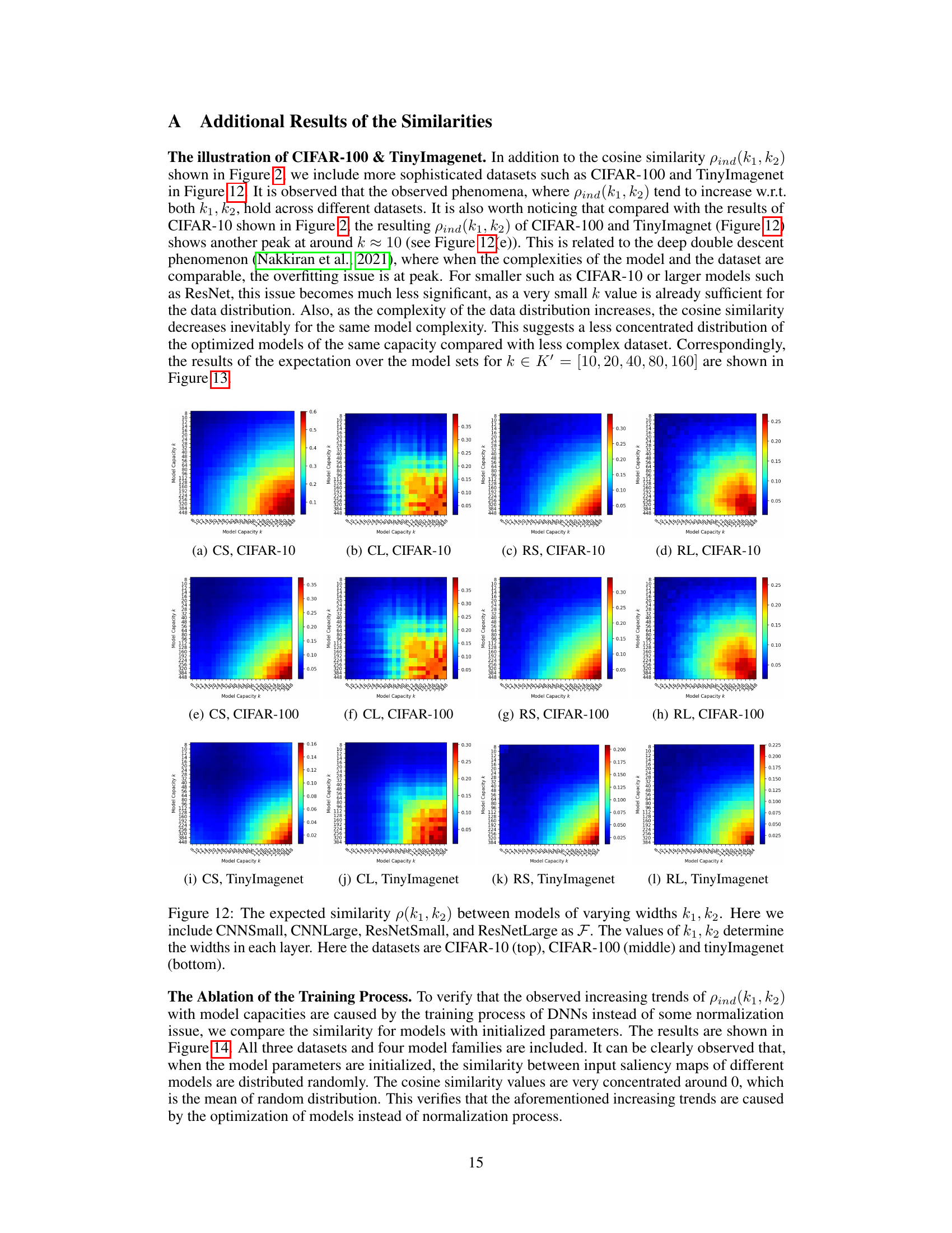
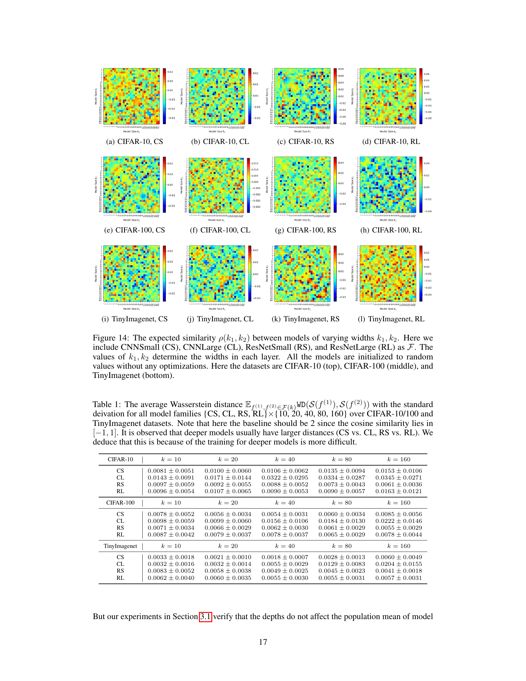
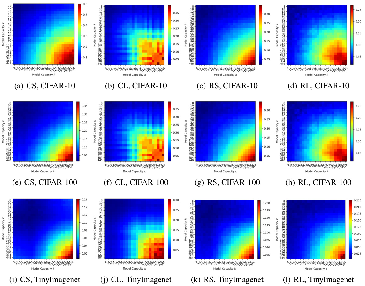
🔼 This figure shows heatmaps representing the expected cosine similarity between input salience maps of two models with different widths (k1 and k2). The models tested belong to four different families (CNNSmall, CNNLarge, ResNetSmall, ResNetLarge), and the experiment is repeated across three different datasets (CIFAR-10, CIFAR-100, TinyImagenet). Each heatmap cell represents the expected similarity between models from families with widths k1 and k2. The color intensity indicates the degree of similarity (higher intensity means higher similarity). This figure visually demonstrates the hypothesis that the similarity between models increases as the model width (capacity) increases, and this behavior is consistent across different model architectures and datasets.
read the caption
Figure 12: The expected similarity p(k1,k2) between models of varying widths k1,k2. Here we include CNNSmall, CNNLarge, ResNetSmall, and ResNetLarge as F. The values of k1, k2 determine the widths in each layer. Here the datasets are CIFAR-10 (top), CIFAR-100 (middle) and tinyImagenet (bottom).

🔼 This figure illustrates two scenarios of the directional gradient distribution of stochastically optimized models. (a) shows a random distribution where different model families (represented by different colors) are not closely related. (b) shows a convergent distribution, where model families align more as model capacity increases, supporting the hypothesis of the paper.
read the caption
Figure 1: A synthetic illustration of the distribution of the directional gradients of stochastically optimized models of the same input data. The subfigures demonstrate (a) an intuitive, stochastic scenario, where the distributions of different model families are not closely dependent, and (b) the converging distribution trend introduced by our hypothesis. Different colors represent different model families, and points represent different optimized models.

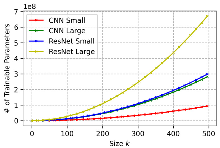
🔼 This figure shows the number of trainable parameters for different model architectures (CNN Small, CNN Large, ResNet Small, ResNet Large) as a function of the width parameter k. It illustrates how the model size dramatically increases with increasing k, especially for the larger ResNet models.
read the caption
Figure 16: The # of trainable parameters of models vs. the width parameter k for each architecture.

🔼 This figure illustrates two scenarios of the distribution of directional gradients of stochastically optimized models. The left subfigure shows an intuitive scenario where distributions of different model families are independent, while the right shows the converging distribution trend hypothesized in the paper. Each color represents a different model family, and each point represents a different optimized model.
read the caption
Figure 1: A synthetic illustration of the distribution of the directional gradients of stochastically optimized models of the same input data. The subfigures demonstrate (a) an intuitive, stochastic scenario, where the distributions of different model families are not closely dependent, and (b) the converging distribution trend introduced by our hypothesis. Different colors represent different model families, and points represent different optimized models.

🔼 This figure provides a synthetic illustration to visualize the hypothesis of the paper regarding the distribution of input salience maps. (a) shows a random distribution where different model families (different colors) are not closely related, and (b) illustrates a convergent distribution where different model families tend to align in terms of their population mean directions as model capacity increases. This illustrates the paper’s main hypothesis about the universal convergence trend of input salience.
read the caption
Figure 1: A synthetic illustration of the distribution of the directional gradients of stochastically optimized models of the same input data. The subfigures demonstrate (a) an intuitive, stochastic scenario, where the distributions of different model families are not closely dependent, and (b) the converging distribution trend introduced by our hypothesis. Different colors represent different model families, and points represent different optimized models.

🔼 This figure uses synthetic data to illustrate two scenarios of the distribution of directional gradients from stochastically optimized models. (a) shows a typical stochastic scenario where models from different families (represented by different colors) have independent distributions. (b) illustrates the authors’ hypothesis that distributions converge towards their shared population mean as model capacity increases.
read the caption
Figure 1: A synthetic illustration of the distribution of the directional gradients of stochastically optimized models of the same input data. The subfigures demonstrate (a) an intuitive, stochastic scenario, where the distributions of different model families are not closely dependent, and (b) the converging distribution trend introduced by our hypothesis. Different colors represent different model families, and points represent different optimized models.

🔼 This figure compares three different attack strategies on deep neural networks (DNNs): 1. Single-model attack from the largest model (red): This uses the gradients from the largest model (highest capacity) in the model family to generate adversarial examples. 2. Single-model attack from the same capacity (green): This uses gradients from a model with the same capacity as the target model to generate adversarial examples. This is a control to isolate the effect of the capacity differences on the attack. 3. Attack by the mean direction (blue): This attack leverages the average of gradient directions across multiple models of the same capacity. This explores if averaging gradient directions improves the attack’s transferability, and aims to test the impact of the hypothesis that gradient directions across models converge as model capacity increases. The x-axis represents the capacity of the target model being attacked, and the y-axis represents the success rate of the attack (lower values indicate more successful attacks). The figure aims to demonstrate the effectiveness of using the mean gradient direction for black-box attacks, showing that it significantly outperforms attacks generated from individual models. This supports the paper’s hypothesis about the convergence of gradient directions across model families with increasing capacity.
read the caption
Figure 11: The comparison between the single-model attack from the largest model (red), the single-model attack from the very same capacity (green) and the attack by the mean direction (blue).

🔼 This figure shows the cosine similarity between CNNs and ResNets with different batch sizes. The cosine similarity is a measure of the similarity between the input salience maps of two models. As can be seen, the cosine similarity increases as the batch size increases. The figure also shows the training loss and accuracy for the models with different batch sizes. The loss decreases as the batch size increases, while the accuracy increases.
read the caption
Figure 18: (a) and (b) illustrate the cosine similarity between (a) CNNs and (b) ResNets with different batch sizes in {64, 128, 256, 512}. (c) shows the loss and (d) shows the accuracy of trained models.

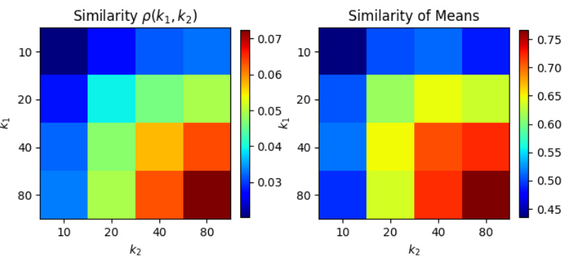
🔼 This figure shows the results of experiments on Vision Transformers (ViTs) trained on CIFAR-10 dataset. The model capacity is varied by changing the embedding dimension (4k), which is separated into k/2 heads. The figure consists of two heatmaps. The left heatmap displays the average cosine similarity between pairs of models with different capacities (k1 and k2). The right heatmap shows the cosine similarity between the mean salience directions of models with different capacities.
read the caption
Figure 21: The cosine similarity between Vision Transformers (ViTs) on CIFAR-10. The capacity is controlled by k ∈ {10, 20, 40, 80}, where the embedding dimension is 4k, separated to k/2 heads. The left subfigure shows the mean of the similarity. The right subfigure shows the similarity of the population mean.

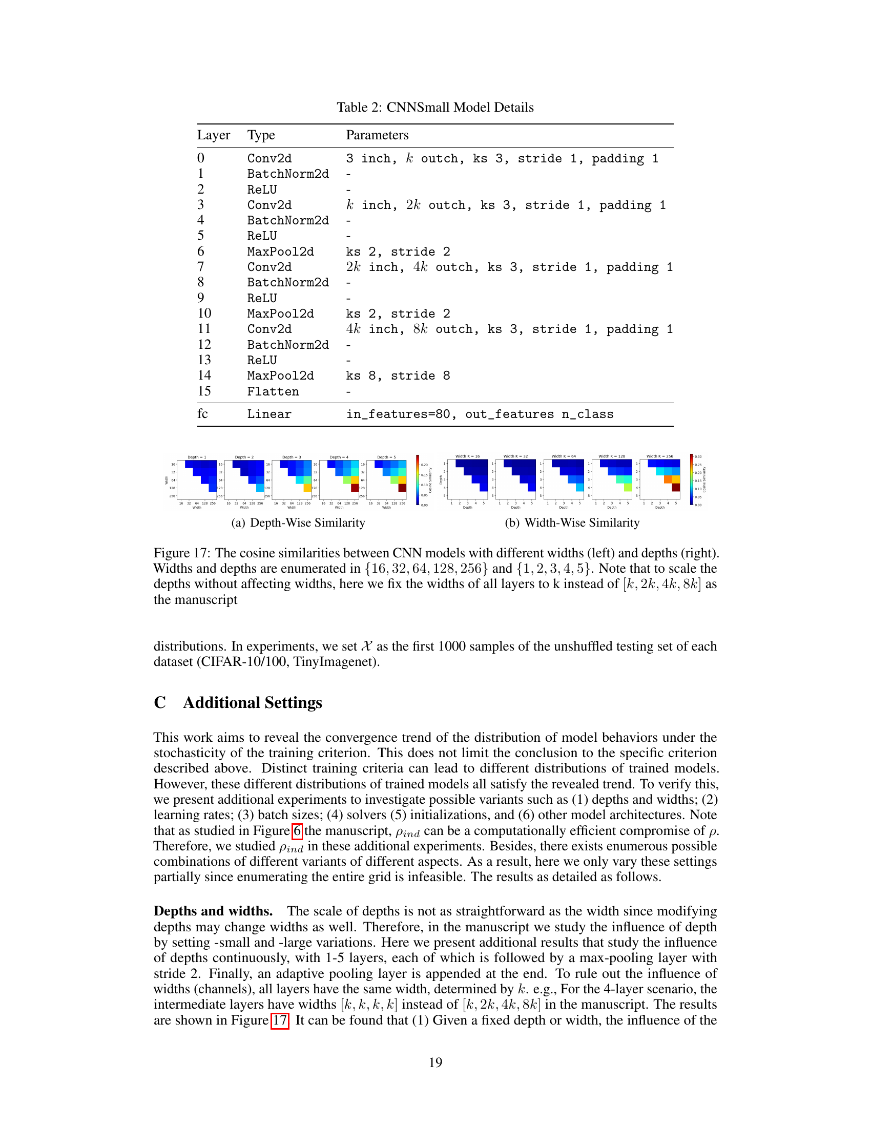
🔼 This figure shows the cumulative distribution function (CDF) of the cosine similarity between two independent, high-dimensional Gaussian vectors for different dimensions (d = 3, 192, 3072). It demonstrates how the probability of observing a high cosine similarity decreases dramatically as the dimensionality increases. In high-dimensional spaces, the cosine similarity is highly concentrated around zero, indicating a low probability of randomly sampled vectors having large cosine similarity. This result is important because the cosine similarity is directly related to the study’s measure of input salience similarities.
read the caption
Figure 22: The relation between the probability P(Z > p) and the cosine similarity value p.

🔼 This figure shows the individual similarity between input salience of two stochastically optimized models, f(1) and f(2), which belong to model families F(k1) and F(k2) respectively, with varying capacities k1 and k2. The similarity is calculated as the cosine similarity of input gradients averaged over the entire test set. The experiment is performed using CIFAR-10 and CIFAR-100 datasets and two different model architectures: CNN and ResNet. The figure aims to illustrate how the similarity of input salience between two models changes with respect to their capacities.
read the caption
Figure 2: The individual similarity pind(f(1), f(2)) = Ex∈x[CosSim(∇æ f(1)(x), ∇æ f(2)(x))], where f(1) ∈ F(k1), f(2) ∈ F(k2). CIFAR-10/100 and CNN & ResNets are tested here.

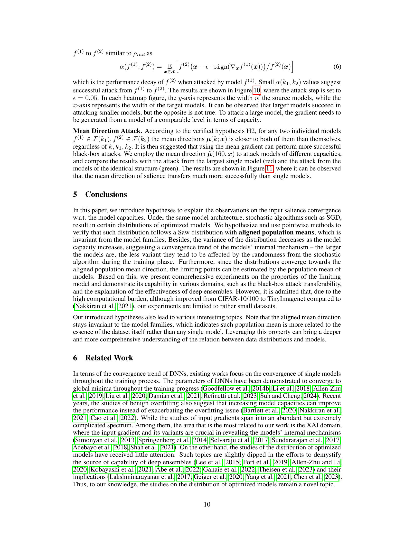
🔼 This figure shows the correlation between the expected testing loss and the marginal expectation of t for both single models and deep ensembles, using CIFAR-100 and TinyImagenet datasets. The plots demonstrate that as the marginal expectation of t (a measure of gradient alignment) increases, the testing loss generally decreases, indicating a relationship between gradient alignment and model performance. Different colors and shapes represent different model families and the capacity of the models. This figure supports the authors’ hypothesis about the convergence trend of input salience and its relationship to model performance.
read the caption
Figure 24: The illustration of the relation between the expected testing loss Ex[L] and the marginal expectation Ex[t]. Both (a) CIFAR-100 and (b) TinyImagenet results are shown as supplementary to Figure 9. Models are from (i) single models with varying structure; and (ii) deep ensembles with varying members. Each color represents a model family.

🔼 This figure shows the results of a single model black-box attack where the adversarial samples are generated from the gradients of source models. The y-axis shows the width of the source models, while the x-axis shows the width of the target models. The color of each entry represents the attack success rate, with darker colors indicating higher success rates.
read the caption
Figure 25: The results of single model black-box attack. The value of each entry is α(k₁, k₂) for different model capacities, where k₁ is the width parameter of the source model and k₂ is the width parameter of the target model.

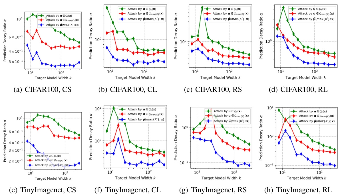
🔼 This figure compares three different black-box attack strategies on various model architectures (CNNs and ResNets) using CIFAR-10 datasets. The attacks target models of different capacities (width). The attack strategies are: (1) using the gradient from the largest trained model (red), (2) using gradients from models of the same capacity as the target model (green), and (3) using the mean gradient direction across models of different capacities (blue). The y-axis represents the attack success rate, and the x-axis represents the capacity of the target model. The results show that using the mean gradient direction consistently outperforms the other two attack strategies, highlighting its effectiveness in the black-box setting.
read the caption
Figure 11: The comparison between the single-model attack from the largest model (red), the single-model attack from the very same capacity (green) and the attack by the mean direction (blue).

TL;DR#

Key Takeaways#

Why does it matter?#

Visual Insights#

In-depth insights#

DNN Salience Trends#

Convergence Analysis#

Saw Dist. Modeling#

Black-box Attack#

Deep Ensemble#

More visual insights#

Full paper#