TL;DR#
Deep equilibrium models (DEQ) offer superior parameter efficiency but suffer from high computational costs during inference due to iterative fixed-point calculations. Existing acceleration strategies, like fixed-point reuse and early stopping, address this issue inefficiently by applying uniform controls across all dimensions. This paper identifies the phenomenon of ‘heterogeneous convergence’, where different dimensions converge at different speeds. This phenomenon is exploited by DeltaDEQ to selectively skip computation in already-converged dimensions.
DeltaDEQ introduces a delta updating rule that caches intermediate linear operation results, recalculating only if activation changes exceed a threshold. Experiments show remarkable FLOPs reduction (84% for INR, 73-76% for optical flow) across various datasets while maintaining accuracy comparable to full-update DEQ models. The method proves orthogonal to existing acceleration techniques and generalizes beyond DEQ models. The code is publicly available.
Key Takeaways#
Why does it matter?#
This paper is crucial for researchers working with implicit neural networks and iterative methods. It introduces a novel acceleration technique, DeltaDEQ, significantly reducing computation costs during inference without compromising accuracy. This is highly relevant to the ongoing quest for more efficient deep learning models, offering potential improvements across various applications.
Visual Insights#
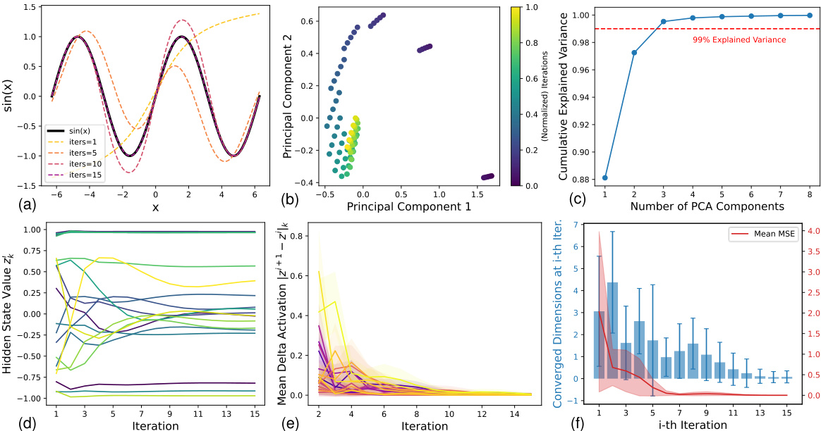
🔼 This figure visualizes several key observations supporting the concept of heterogeneous convergence in deep equilibrium models. Subfigure (a) shows the model’s reconstruction improving with more iterations. (b) displays the hidden state trajectory using PCA, indicating lower dimensionality than expected. (c) further supports this with cumulative explained variance. (d) and (e) illustrate the varying convergence speeds across different dimensions of the hidden state. Finally, (f) shows how many dimensions converge at each iteration and the overall model error.
read the caption
Figure 1: (a) Reconstruction evolution when increasing inference iterations. (b) Hidden states trajectory for 5 consecutive input points with the first two principal components. Details in A.1. (c) Cumulative explained variance for all hidden states. (d) Evolution of different dimensions of hidden states (represented by colors) over iterations. (e) Mean delta activation for different dimensions (represented by colors). The colored solid areas indicate the standard deviation from different inputs. (f) Histogram of converged dimensions (blue) at i-th iteration and evolution of the model prediction MSE (red).

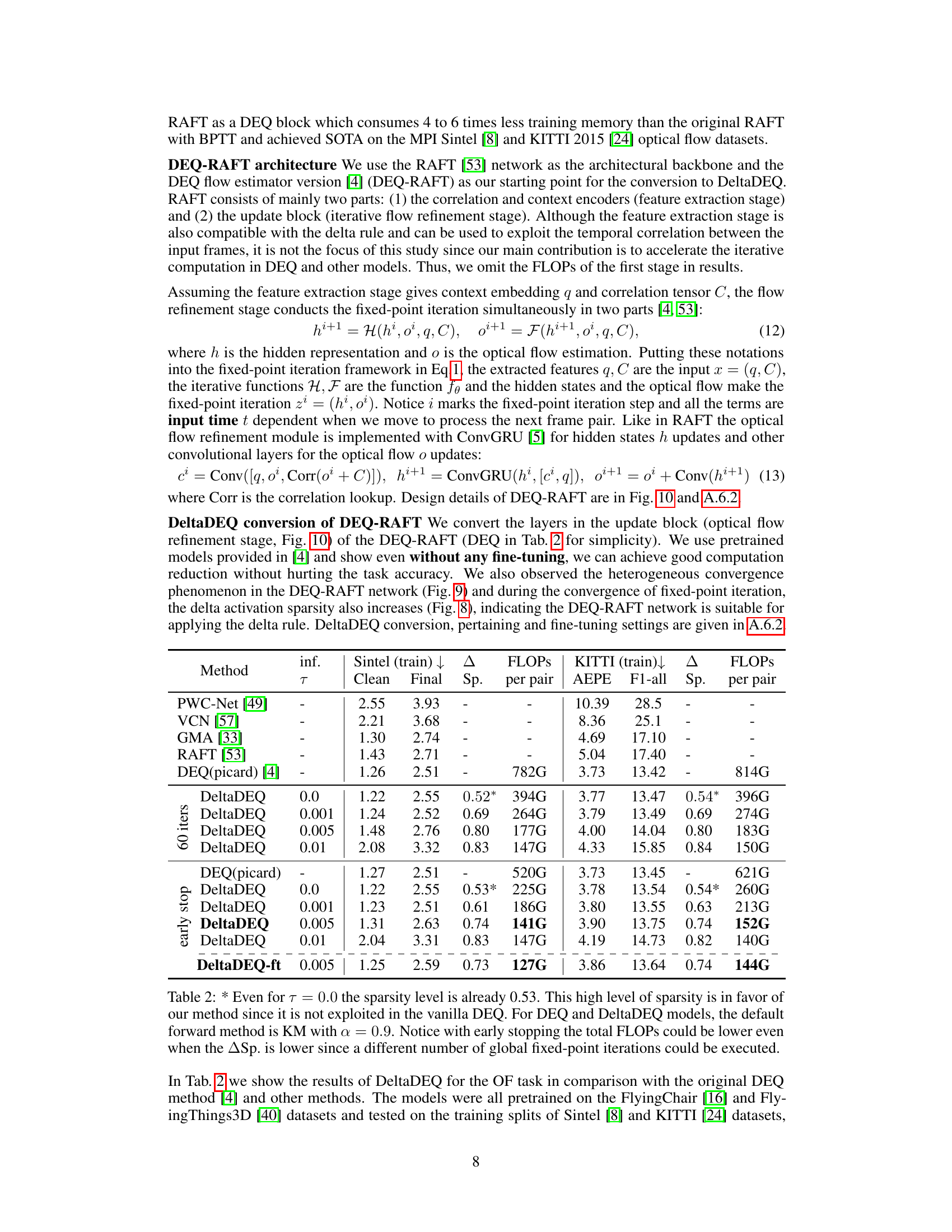
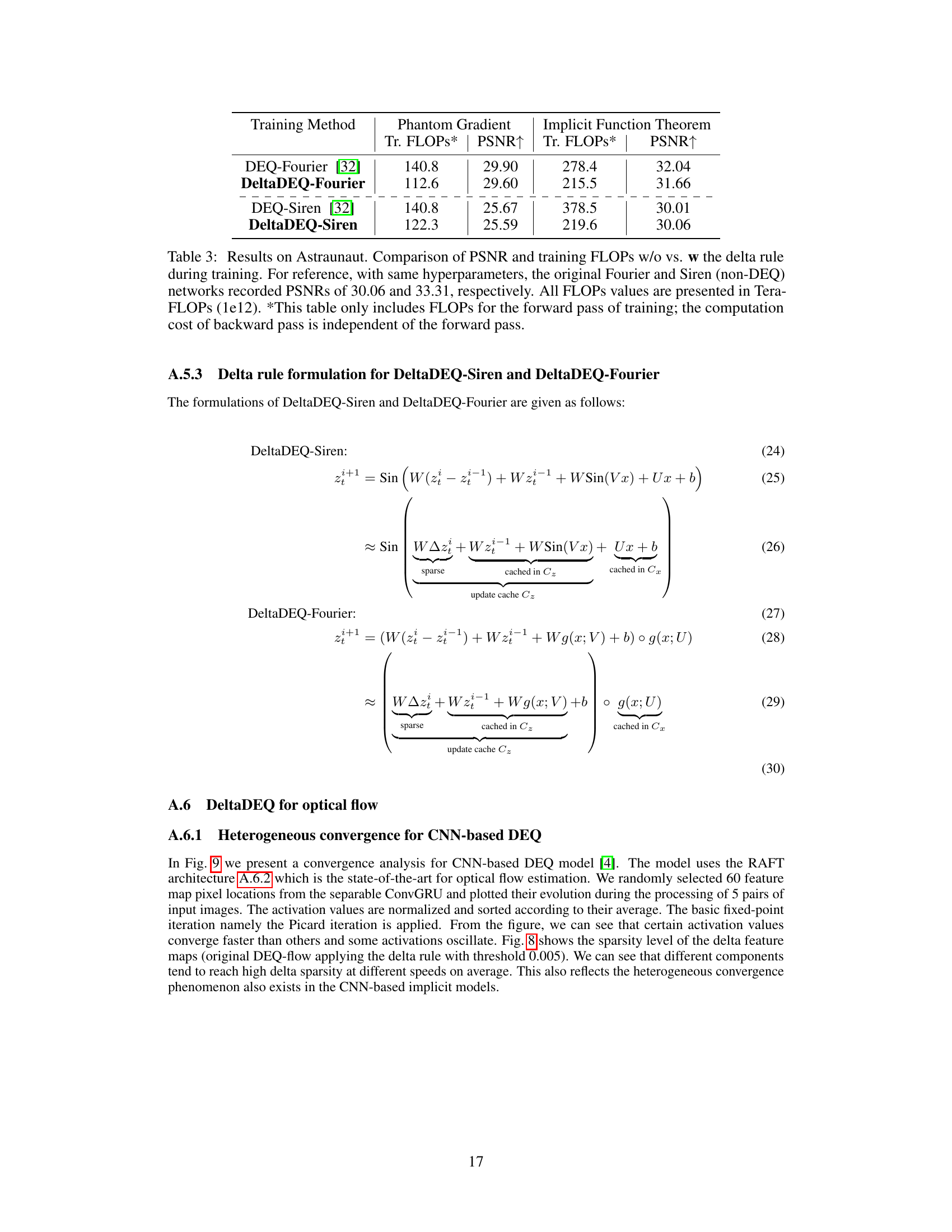
🔼 This table compares the Peak Signal-to-Noise Ratio (PSNR) and training FLOPs (floating point operations) of DEQ-Fourier and DEQ-Siren models with and without the delta rule applied during training. It shows the reduction in FLOPs achieved by DeltaDEQ while maintaining comparable PSNR. Note that only the FLOPs of the forward pass are included, as the backward pass computation is independent.
read the caption
Table 1: Comparison of PSNR and training FLOPs w/o vs. w the delta rule during training. For reference, with same hyperparameters, the original Fourier and Siren (non-DEQ) networks recorded PSNRs of 30.06 and 33.31, respectively. All FLOPs values are presented in Tera-FLOPs (1e12). *This table only includes FLOPs for the forward pass of training; the computation cost of backward pass is independent of the forward pass.
In-depth insights#
DeltaDEQ: Heterogeneous Convergence#
The concept of “DeltaDEQ: Heterogeneous Convergence” introduces a novel approach to accelerate deep equilibrium model (DEQ) training and inference. It leverages the observation that different dimensions of the hidden state converge at varying speeds during iterative updates in DEQs. This heterogeneity is then exploited by DeltaDEQ via a sparse update mechanism, where computations are skipped for dimensions already deemed converged, leading to significant FLOPs reduction. The key is identifying and utilizing this asynchronous convergence behavior to optimize the computational cost of the fixed-point iteration. DeltaDEQ’s effectiveness is empirically demonstrated across diverse tasks, showcasing its potential for broader applications in implicit neural networks and iterative methods generally. The method appears particularly efficient when combined with other acceleration techniques, such as fixed-point reuse.
Delta Rule Acceleration#
Delta Rule Acceleration is a novel method to enhance computational efficiency in deep equilibrium models by leveraging the heterogeneous convergence phenomenon. The core idea is that different dimensions of the hidden state converge at varying speeds. By identifying and exploiting this disparity, Delta Rule Acceleration selectively skips computations for already-converged dimensions. This is achieved through a delta updating rule, storing past linear operations and propagating state activations only when changes exceed a threshold. This method shows substantial FLOPs reduction across various tasks like implicit neural representation and optical flow estimation while maintaining comparable accuracy. The method’s orthogonality to existing acceleration techniques like fixed-point reuse makes it a valuable addition to the DEQ model optimization arsenal. Further research should explore the method’s effectiveness across a wider range of architectures and datasets, potentially leading to even greater improvements in computational efficiency.
INR & OF Experiments#
The ‘INR & OF Experiments’ section likely details the application of the proposed DeltaDEQ method to two distinct tasks: Implicit Neural Representation (INR) and Optical Flow (OF) estimation. INR experiments would probably involve training DeltaDEQ on image datasets to reconstruct images from input coordinates, comparing its performance (reconstruction quality, computational efficiency) against existing INR techniques. Optical flow experiments would focus on evaluating DeltaDEQ’s ability to accurately predict pixel motion between video frames, potentially using benchmarks like Sintel and KITTI. The authors would likely highlight performance improvements offered by DeltaDEQ in terms of FLOPs reduction and speedup while maintaining comparable accuracy to baseline DEQ methods. The discussion would probably analyze the heterogeneous convergence phenomenon within the context of both tasks, showing how DeltaDEQ effectively leverages this characteristic for computational gains. Key metrics for evaluation would likely include PSNR (Peak Signal-to-Noise Ratio) for INR and AEPE (Average Endpoint Error) for OF, along with FLOP counts and inference time comparisons.
Limitations and Future#
The paper’s core contribution, DeltaDEQ, demonstrates significant FLOPs reduction in deep equilibrium models by exploiting heterogeneous convergence. A key limitation is the reliance on sparsity, which may not consistently materialize across diverse datasets or model architectures. While effective in RNN and CNN-based models, the generalization to transformer networks requires further investigation. Hardware practicality for sparse convolutions is another limitation, necessitating specialized hardware for optimal performance gains. Future work should focus on addressing this hardware limitation, potentially through optimized sparse convolution libraries or tailored hardware designs. Furthermore, research into adaptive thresholding mechanisms and more robust sparsity prediction techniques could enhance performance and expand applicability. Investigating DeltaDEQ’s effectiveness in scenarios with temporal correlations beyond video frames is also warranted. Finally, exploring the application of DeltaDEQ to a broader range of implicit models and optimization methods beyond fixed-point iteration is an important direction for future development.
Related Works#
The ‘Related Works’ section would ideally delve into existing acceleration techniques for implicit neural networks, contrasting and comparing them to the proposed DeltaDEQ method. It should discuss methods that exploit temporal correlations in input data, such as fixed-point reuse or early stopping, highlighting their limitations and how DeltaDEQ addresses them. A detailed comparison with other sparsity-inducing techniques, such as layer skipping or activation pruning, would provide valuable context, emphasizing DeltaDEQ’s unique focus on heterogeneous convergence and its ability to achieve sparsity without sacrificing expressiveness. Furthermore, a thorough analysis of existing DEQ models and their limitations regarding computational cost during inference is crucial, illustrating how DeltaDEQ offers a novel approach to overcome these challenges. Finally, the discussion should clearly articulate how DeltaDEQ differs from and improves upon prior work, highlighting its potential advantages and unique contributions to the field.
More visual insights#
More on figures
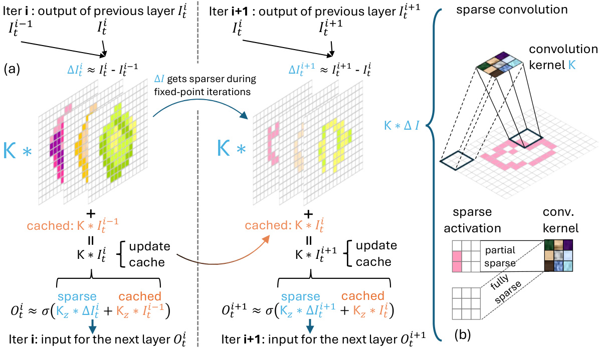
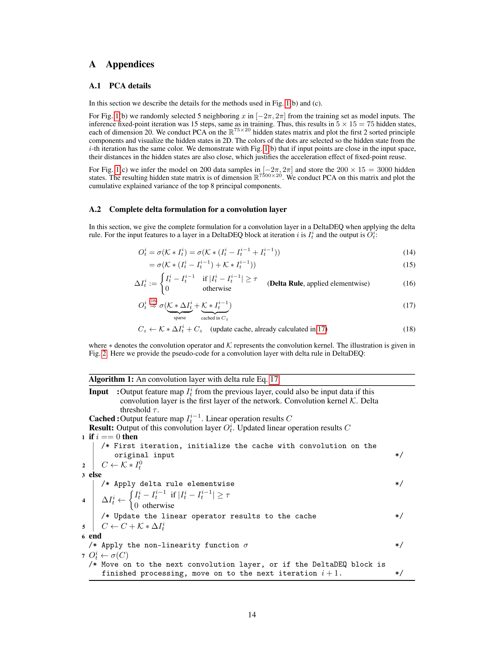
🔼 This figure illustrates the mechanism of DeltaDEQ, a method to leverage heterogeneous convergence for accelerating deep equilibrium iterations. Panel (a) shows how the input from the previous iteration (It-1) is stored and subtracted from the current iteration’s input (It) to create a sparse delta (ΔI). This sparsity increases with each iteration. Panel (b) details how this sparse delta is used in sparse convolutions, allowing for computational savings by skipping computations on zero entries. The figure highlights the efficiency gains achievable through this method.
read the caption
Figure 2: (a) Convolution type of DeltaDEQ. The input I¯¹ from the previous iteration is stored and subtracted to create the sparse ∆Ι. White represents zero. (b) For sparse convolution, in theory, all zero entries in the feature map can be skipped; in practice, this is more feasible on hardware [1, 15] when the entire activation patch is fully sparse. The complete formulation and pseudo-code are given in A.2 and RNN type DeltaDEQ is illustrated in A.5.1.

🔼 This figure visualizes several key observations about the heterogeneous convergence phenomenon in deep equilibrium models. Subfigure (a) shows the model’s reconstruction improving with more inference iterations. Subfigure (b) displays the trajectory of hidden states in a 2D PCA projection, demonstrating that similar inputs lead to nearby hidden state trajectories. Subfigure (c) shows that a small number of principal components capture most of the variance in hidden states. Subfigures (d) and (e) illustrate the heterogeneous convergence, where some dimensions converge much faster than others. Subfigure (f) presents a histogram of converged dimensions at each iteration and the model’s mean squared error (MSE) over time, further demonstrating that the convergence speed varies across dimensions.
read the caption
Figure 1: (a) Reconstruction evolution when increasing inference iterations. (b) Hidden states trajectory for 5 consecutive input points with the first two principal components. Details in A.1. (c) Cumulative explained variance for all hidden states. (d) Evolution of different dimensions of hidden states (represented by colors) over iterations. (e) Mean delta activation for different dimensions (represented by colors). The colored solid areas indicate the standard deviation from different inputs. (f) Histogram of converged dimensions (blue) at i-th iteration and evolution of the model prediction MSE (red).
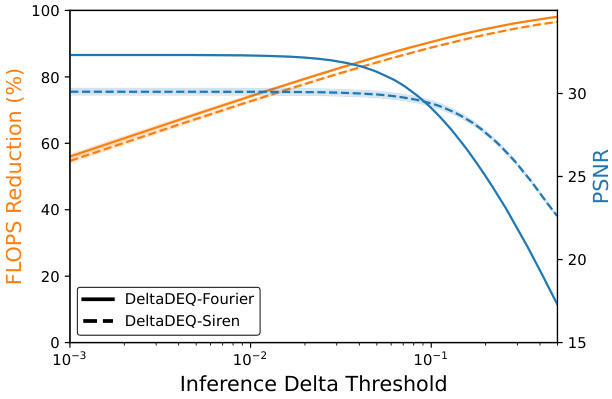
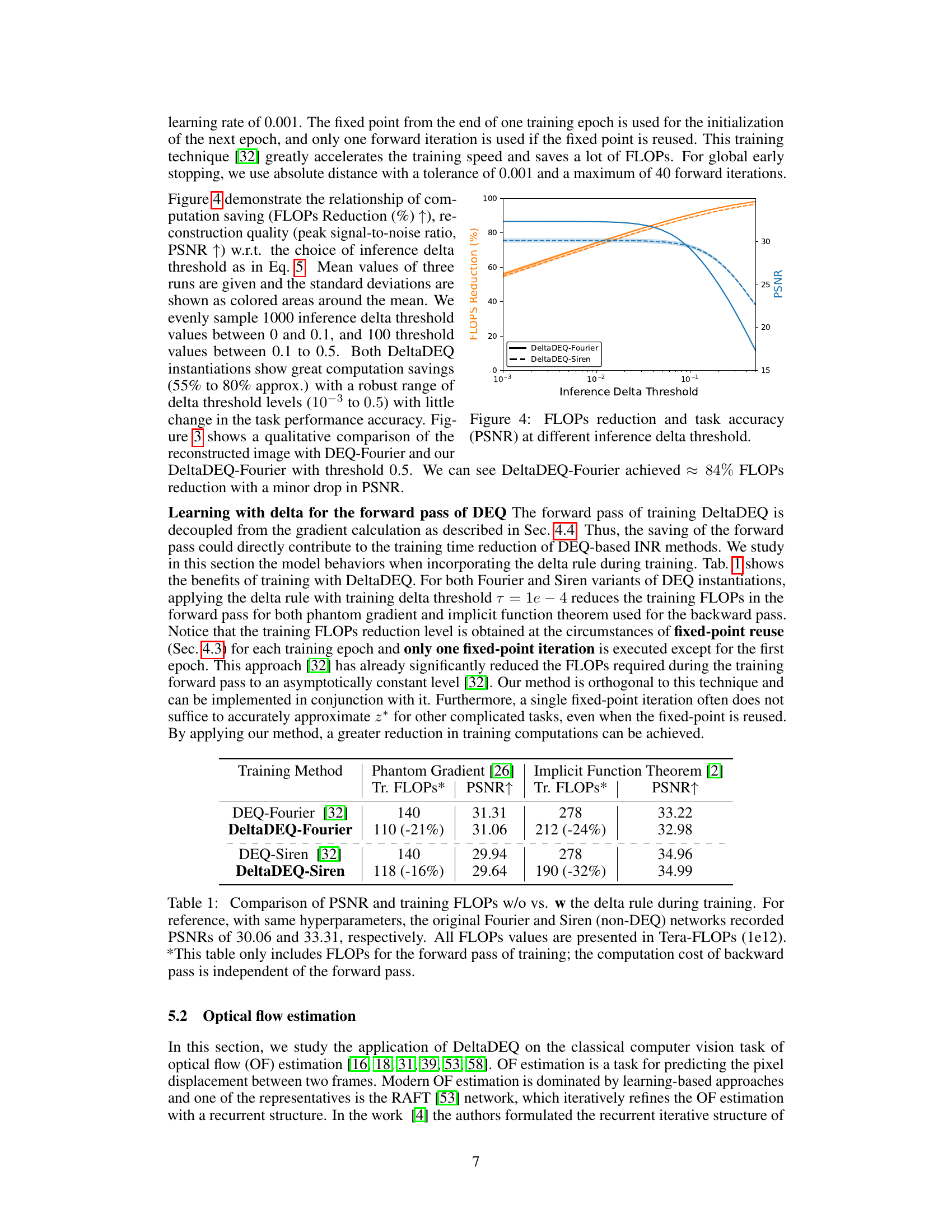
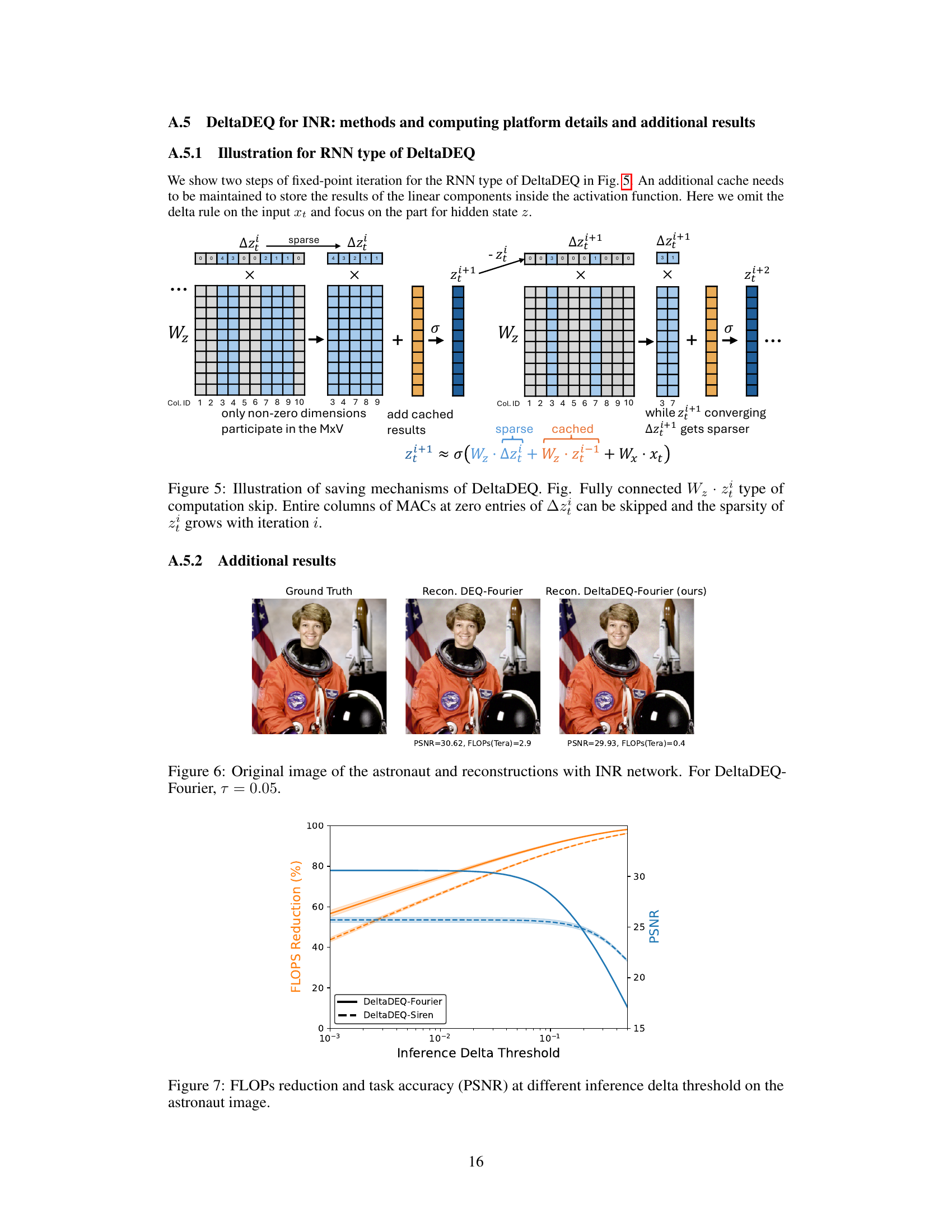
🔼 This figure shows the relationship between computation saving (in terms of FLOPs reduction), reconstruction quality (measured by PSNR), and the inference delta threshold. The results are averaged over three runs, with standard deviations represented as shaded areas. The plot demonstrates a trade-off; increasing the threshold leads to greater FLOPs reduction but potentially at the cost of slightly lower PSNR. The figure illustrates that a range of thresholds provides substantial computation savings while maintaining high reconstruction quality.
read the caption
Figure 4: FLOPs reduction and task accuracy (PSNR) at different inference delta threshold.
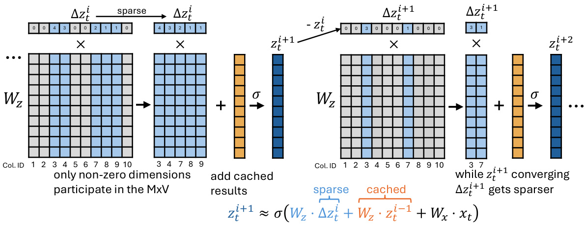
🔼 This figure illustrates how DeltaDEQ saves computation. In a standard RNN layer, a matrix-vector multiplication (MxV) is performed using the full weight matrix (Wz) and the state vector (zi). DeltaDEQ modifies this by calculating the change (∆zi) in the state vector between iterations. Only the non-zero elements of ∆zi participate in the MxV operation, significantly reducing computations. The cached results from the previous iteration are added to further improve efficiency. The figure shows how the sparsity of ∆zi increases as the fixed-point iteration converges, leading to substantial computational savings.
read the caption
Figure 5: Illustration of saving mechanisms of DeltaDEQ. Fig. Fully connected Wz.zi type of computation skip. Entire columns of MACs at zero entries of ∆zi can be skipped and the sparsity of zi grows with iteration i.
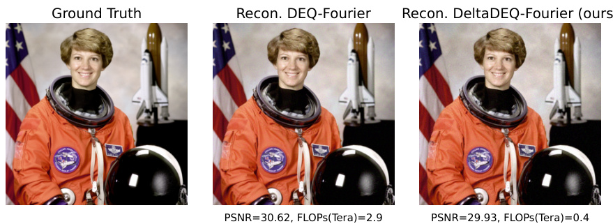
🔼 This figure shows a comparison of the original image and reconstructions obtained using the INR (Implicit Neural Representation) network with different methods. It compares the reconstruction quality of the DEQ-Fourier method and the proposed DeltaDEQ-Fourier method. The PSNR (Peak Signal-to-Noise Ratio) and FLOPs (floating-point operations) for each method are provided, demonstrating the computational savings achieved by the DeltaDEQ-Fourier method.
read the caption
Figure 3: Original image and reconstructions with INR network.
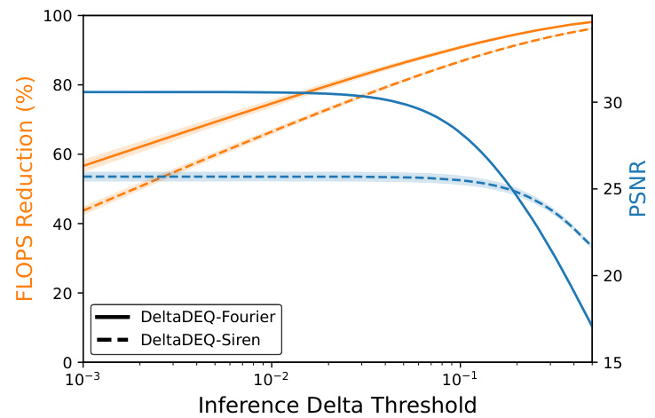
🔼 This figure shows the relationship between computation saving (FLOPs Reduction), reconstruction quality (PSNR), and the inference delta threshold. The x-axis represents the inference delta threshold, while the y-axis shows both FLOPs reduction and PSNR. Two lines represent different DeltaDEQ model architectures: DeltaDEQ-Fourier and DeltaDEQ-Siren. The figure demonstrates the impact of different inference delta thresholds on the model’s performance and computation cost. Each line represents the mean of three runs, and shaded areas show standard deviations.
read the caption
Figure 4: FLOPs reduction and task accuracy (PSNR) at different inference delta threshold.
🔼 This figure visualizes the heterogeneous convergence phenomenon observed in deep equilibrium models. Subfigure (a) shows the model’s reconstruction improving with more iterations. Subfigures (b) and (c) show the dimensionality reduction of hidden states using PCA. Subfigures (d) and (e) show how different dimensions of hidden states converge at different speeds. Subfigure (f) shows the number of converged dimensions and the model’s MSE over iterations.
read the caption
Figure 1: (a) Reconstruction evolution when increasing inference iterations. (b) Hidden states trajectory for 5 consecutive input points with the first two principal components. Details in A.1. (c) Cumulative explained variance for all hidden states. (d) Evolution of different dimensions of hidden states (represented by colors) over iterations. (e) Mean delta activation for different dimensions (represented by colors). The colored solid areas indicate the standard deviation from different inputs. (f) Histogram of converged dimensions (blue) at i-th iteration and evolution of the model prediction MSE (red).
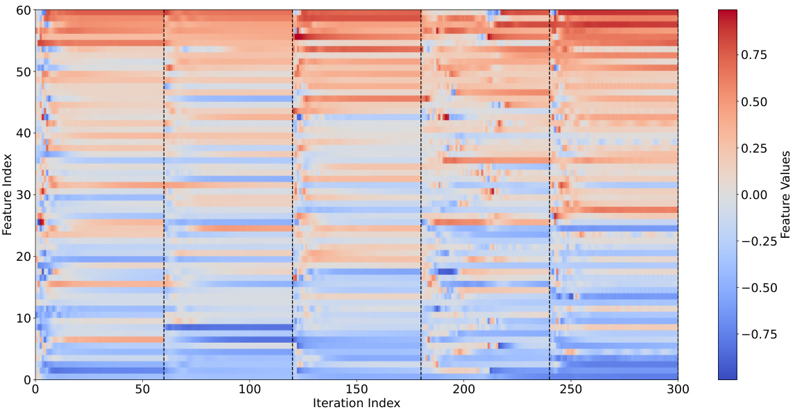
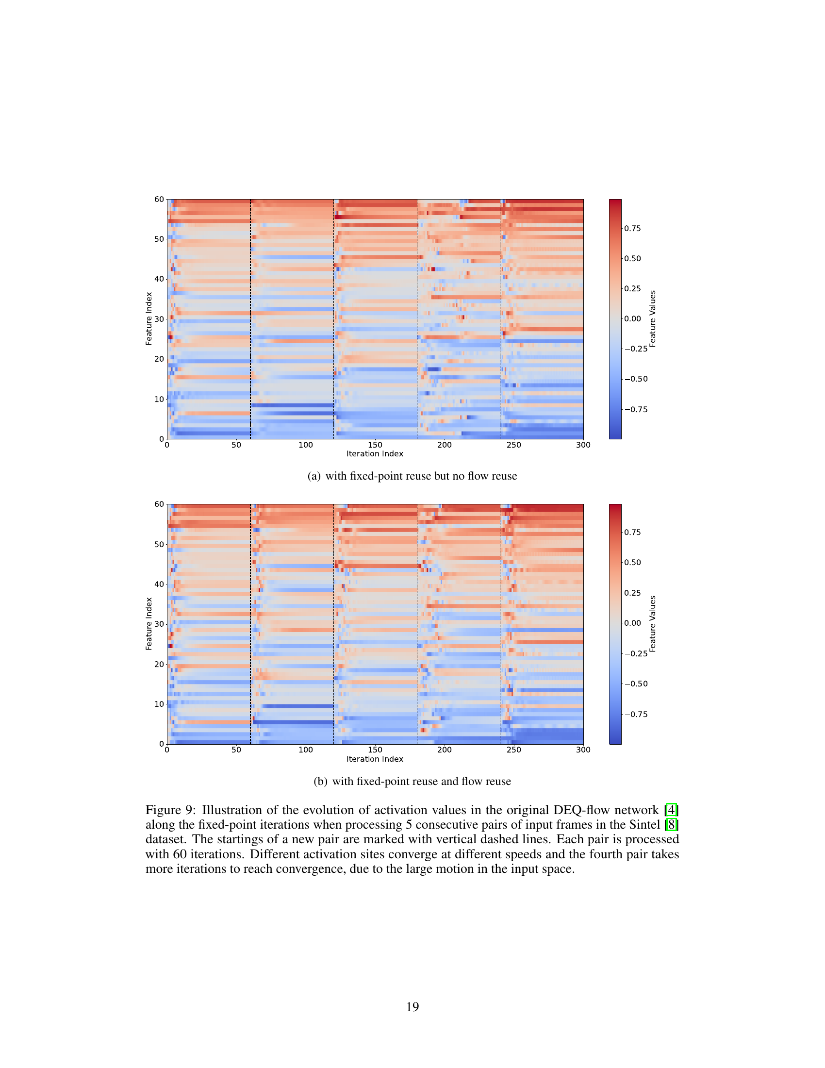
🔼 This figure shows the evolution of activation values in the original DEQ-flow network during fixed-point iterations while processing five consecutive pairs of input frames from the Sintel dataset. Each pair undergoes 60 iterations. The figure highlights that different activation sites converge at varying speeds, with the fourth pair requiring more iterations due to significant motion within the input space.
read the caption
Figure 9: Illustration of the evolution of activation values in the original DEQ-flow network [4] along the fixed-point iterations when processing 5 consecutive pairs of input frames in the Sintel [8] dataset. The startings of a new pair are marked with vertical dashed lines. Each pair is processed with 60 iterations. Different activation sites converge at different speeds and the fourth pair takes more iterations to reach convergence, due to the large motion in the input space.
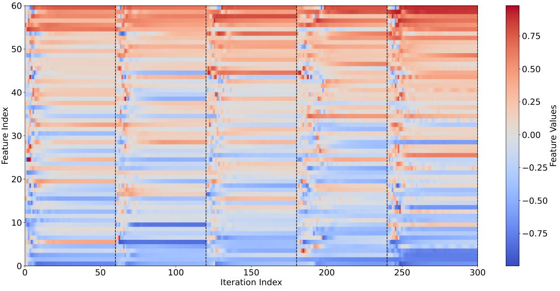
🔼 This figure shows the evolution of activation values in the original DEQ-flow network during fixed-point iterations while processing 5 consecutive pairs of input frames from the Sintel dataset. Each pair undergoes 60 iterations. The start of each new pair is indicated by dashed vertical lines. The figure highlights the heterogeneous convergence, where different activation sites converge at varying speeds; this is particularly evident in the fourth pair, which requires more iterations to converge due to significant motion within the input space.
read the caption
Figure 9: Illustration of the evolution of activation values in the original DEQ-flow network [4] along the fixed-point iterations when processing 5 consecutive pairs of input frames in the Sintel [8] dataset. The startings of a new pair are marked with vertical dashed lines. Each pair is processed with 60 iterations. Different activation sites converge at different speeds and the fourth pair takes more iterations to reach convergence, due to the large motion in the input space.
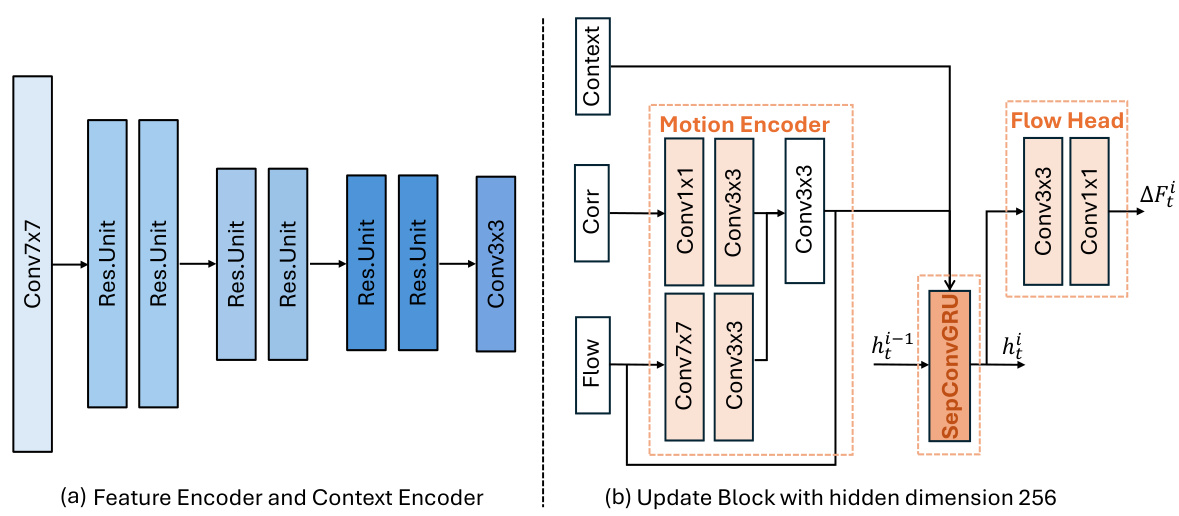
🔼 The figure shows the architecture of RAFT, DEQ-RAFT, and DeltaDEQ for optical flow. It highlights the feature encoder and context encoder, which are common to all three methods. The key difference lies in the update block, which iteratively refines the flow prediction. The DeltaDEQ version incorporates a delta rule to accelerate the computationally intensive update block.
read the caption
Figure 10: Architecture illustration for RAFT [53], DEQ flow [4] and our DeltaDEQ.
More on tables
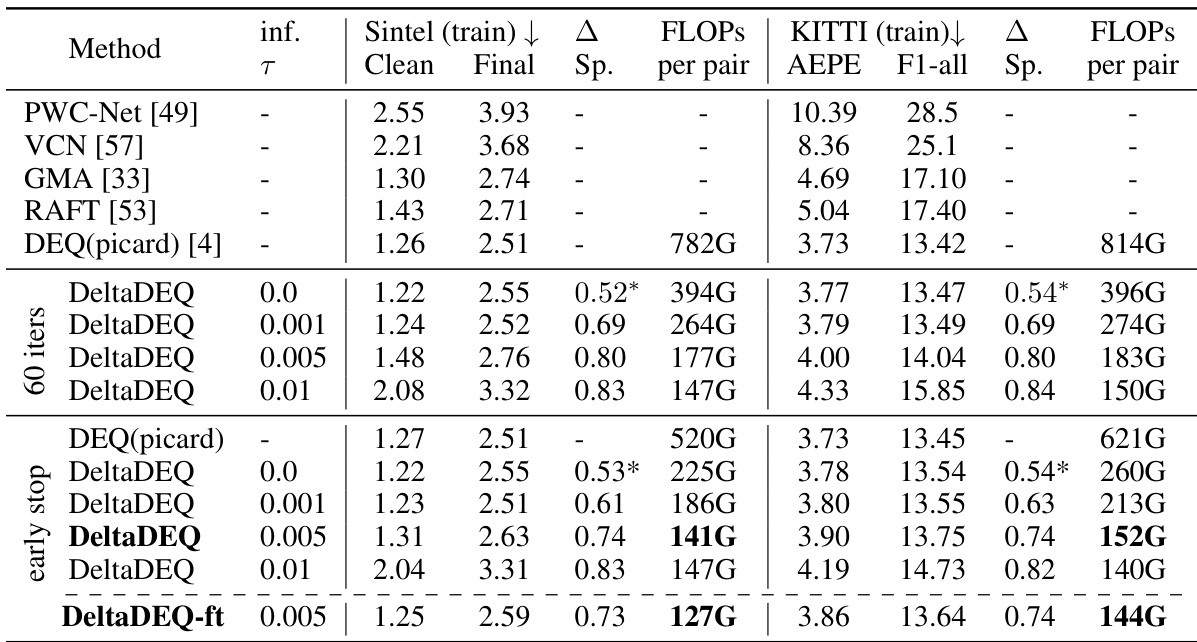
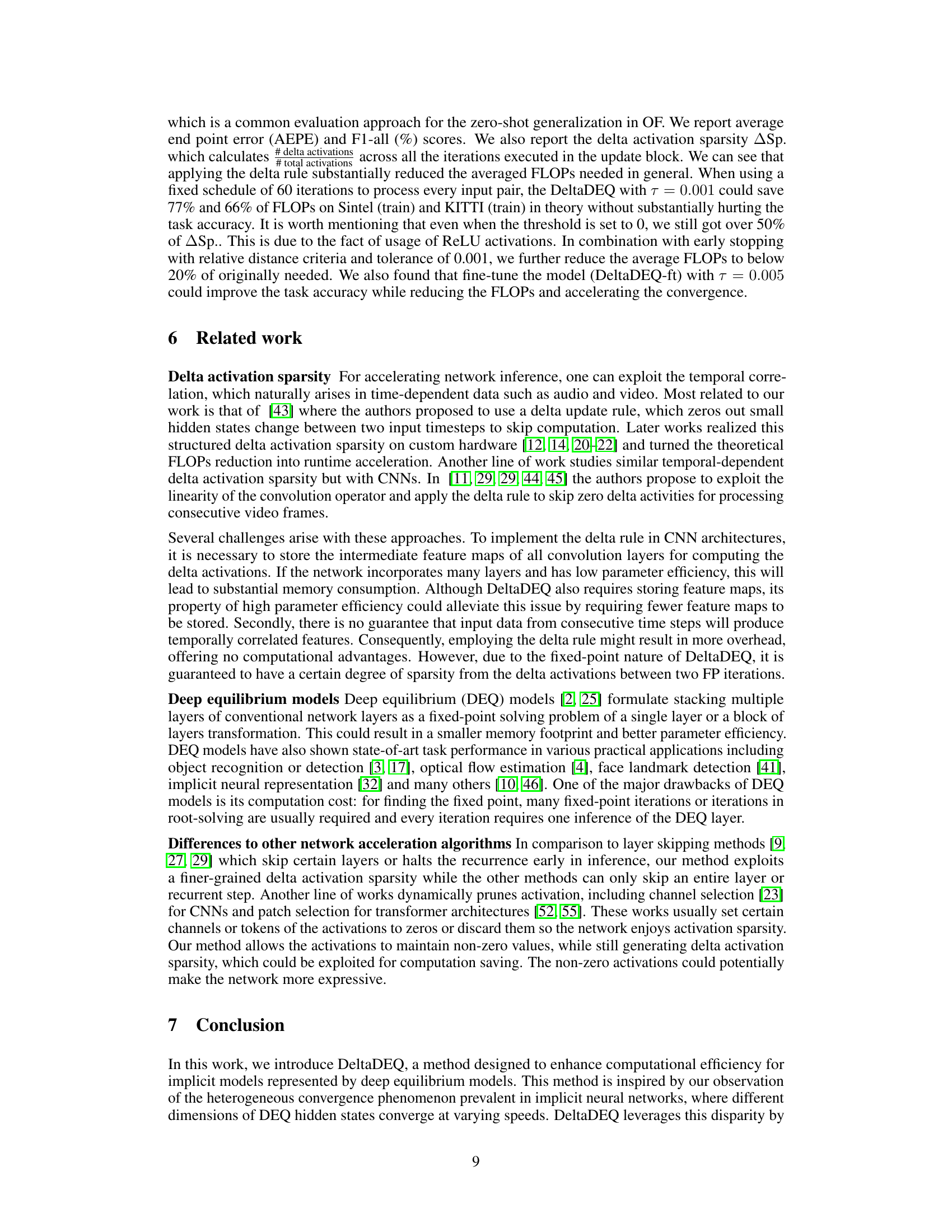
🔼 This table compares different methods for approximating the fixed point in the forward pass of the DEQ-RAFT model for optical flow estimation. It shows the performance (measured by AEPE and F1-all scores) and computational cost (FLOPs) for various methods including Broyden, Anderson, Picard, and Krasnoselskii-Mann (KM) iterations with different numbers of iterations. The results are presented for both the Sintel and KITTI datasets. The asterisk (*) indicates that even with a threshold of 0.0, the sparsity level is high, demonstrating the effectiveness of the DeltaDEQ approach.
read the caption
Table 2: Comparison among different solvers or fixed-point iteration methods for the forward pass.

🔼 This table compares the Peak Signal-to-Noise Ratio (PSNR) and training FLOPs (floating point operations) of DEQ-Fourier and DEQ-Siren models with and without the delta rule applied during training. It also provides a reference PSNR for the original (non-DEQ) Fourier and Siren models for comparison. Note that only the FLOPs for the forward pass during training are included, as the backward pass computation is independent of the forward pass.
read the caption
Table 1: Comparison of PSNR and training FLOPs w/o vs. w the delta rule during training. For reference, with same hyperparameters, the original Fourier and Siren (non-DEQ) networks recorded PSNRs of 30.06 and 33.31, respectively. All FLOPs values are presented in Tera-FLOPs (1e12). *This table only includes FLOPs for the forward pass of training; the computation cost of backward pass is independent of the forward pass.
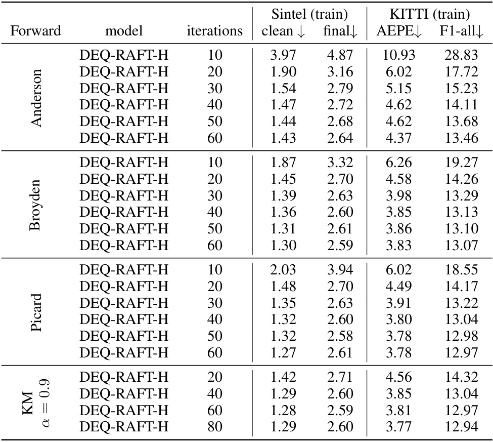
🔼 This table compares the performance of different methods for solving the fixed-point iteration problem in the forward pass of the DEQ-RAFT model. It shows the results for various solvers (Broyden, Anderson, Picard) and fixed-point iterations (KM, Picard) on the Sintel and KITTI datasets. The metrics used to evaluate the performance are clean and final end-point error (AEPE) and F1-all. The number of iterations used for each solver is also shown. This table helps to determine the best method for approximating the fixed point in terms of accuracy and computational efficiency.
read the caption
Table 4: Comparison among different solvers or fixed-point iteration methods for the forward pass.
Full paper#

