TL;DR#
Cooperative multi-agent reinforcement learning (MARL) faces challenges in balancing exploration and exploitation, especially in complex environments. Existing approaches, like those based on Upper Confidence Bounds (UCB), often lack practical efficiency. Randomized exploration strategies, such as Thompson Sampling (TS), offer a promising alternative but have not been extensively explored in cooperative MARL. Moreover, theoretical understanding of their efficiency remains limited.
This research introduces a unified algorithm framework, CoopTS, specifically designed for randomized exploration in parallel Markov Decision Processes (MDPs). Two TS-based algorithms, CoopTS-PHE and CoopTS-LMC, are developed using Perturbed-History Exploration (PHE) and Langevin Monte Carlo (LMC) respectively. The paper provides the first theoretical analysis of provably efficient randomized exploration strategies in cooperative MARL, proving regret bounds and communication complexities for a class of linear parallel MDPs. Extensive experiments, including deep exploration problems, a video game, and real-world energy systems, demonstrate CoopTS’s superior performance, even with model misspecification.
Key Takeaways#
Why does it matter?#
This paper is crucial because it presents the first study on provably efficient randomized exploration in cooperative multi-agent reinforcement learning (MARL). This is a significant advancement as exploration-exploitation balance is a major challenge in MARL, particularly in cooperative settings where coordination among agents is essential. The work provides both theoretical guarantees and strong empirical evidence, opening avenues for more efficient and robust MARL algorithms.
Visual Insights#

🔼 The figure compares the performance of different exploration strategies (PHE, LMC, DQN, Bootstrapped DQN, NoisyNet DQN, DDQN) across four different environments. The first two subfigures (a) and (b) show results from the N-chain environment with chain length N=25 and varying numbers of agents (m=2 and m=3 respectively). The last two subfigures (c) and (d) show results from a Super Mario Bros environment in parallel and federated settings. All results are averaged over 10 runs, and shaded areas represent standard deviations, indicating the variability in the results.
read the caption
Figure 1: Comparison among different exploration strategies in different environments. (a)-(b): N-chain with N = 25. (c)-(d): Super Mario Bros. All results are averaged over 10 runs and the shaded area represents the standard deviation.

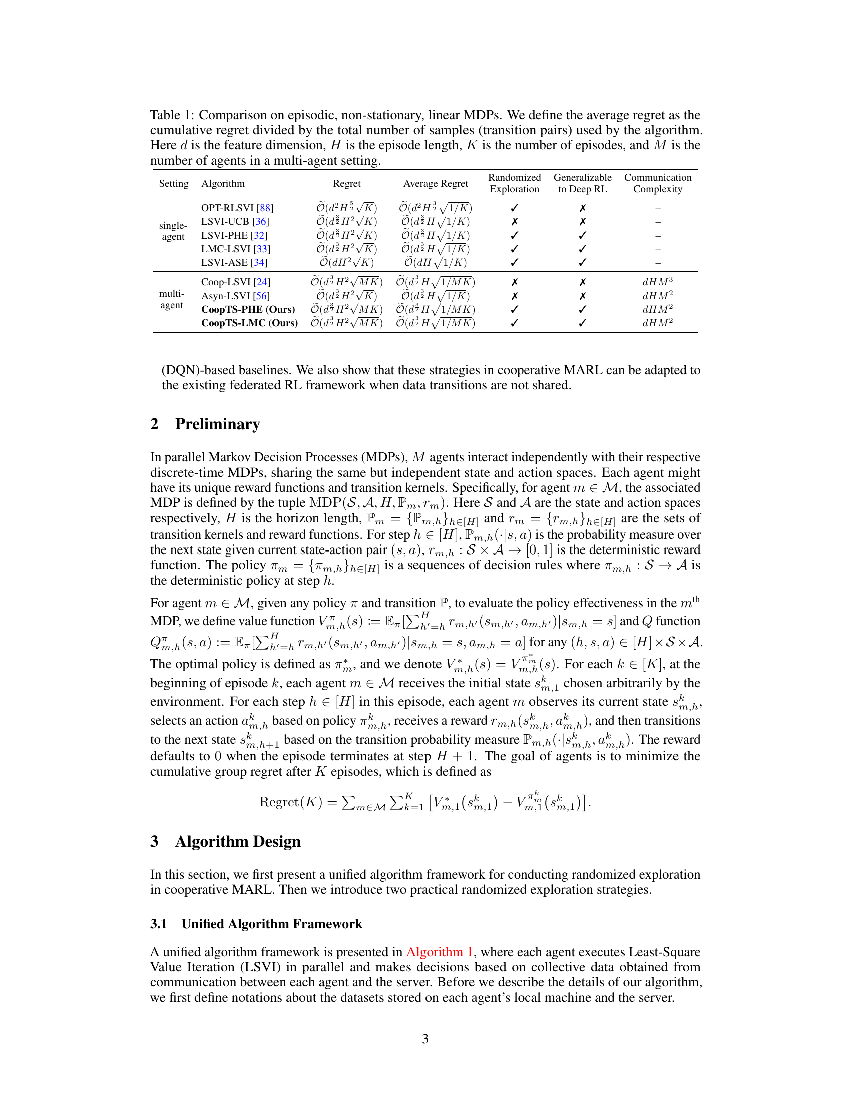
🔼 This table compares the performance of various algorithms (including the authors’ proposed CoopTS-PHE and CoopTS-LMC) on episodic, non-stationary, linear Markov Decision Processes (MDPs). It shows the theoretical regret bounds, average regret, whether the algorithm uses randomized exploration, generalizability to deep reinforcement learning, and communication complexity for both single-agent and multi-agent settings. The table highlights the superior performance of the authors’ methods in terms of regret and communication complexity.
read the caption
Table 1: Comparison on episodic, non-stationary, linear MDPs. We define the average regret as the cumulative regret divided by the total number of samples (transition pairs) used by the algorithm. Here d is the feature dimension, H is the episode length, K is the number of episodes, and M is the number of agents in a multi-agent setting.
In-depth insights#
MARL Exploration#
Multi-agent reinforcement learning (MARL) exploration strategies are crucial for efficient learning in cooperative settings. Randomized exploration methods such as Thompson Sampling (TS) offer advantages over traditional methods like Upper Confidence Bounds (UCB) by avoiding premature convergence to suboptimal policies. The paper explores TS variants like perturbed-history exploration (PHE) and Langevin Monte Carlo (LMC) within a unified framework for parallel Markov Decision Processes (MDPs). Theoretical analysis focuses on regret bounds and communication complexity, demonstrating that the proposed approaches achieve provably efficient exploration, especially in linear MDPs. Empirical evaluations across diverse environments, including N-chains and Super Mario Bros., showcase superior performance compared to existing deep Q-networks and other exploration strategies. Federated learning is also integrated, adapting the framework to scenarios where direct data sharing is restricted. The results highlight the potential of randomized exploration and the unified framework for solving real-world cooperative MARL problems.
CoopTS Algos#
The heading “CoopTS Algos” likely refers to a section detailing the proposed cooperative Thompson Sampling algorithms. These algorithms, likely named CoopTS-PHE and CoopTS-LMC, seem to address the challenge of exploration in cooperative multi-agent reinforcement learning (MARL). CoopTS-PHE integrates the perturbed-history exploration (PHE) strategy, introducing randomness in the action history to diversify experiences. CoopTS-LMC utilizes the Langevin Monte Carlo (LMC) method, employing approximate sampling for efficient exploration. The algorithms are presented as being flexible, easy to implement, and theoretically grounded for a class of linear parallel MDPs. A key aspect appears to be a unified algorithmic framework for learning in parallel MDPs, likely involving communication mechanisms to balance exploration and exploit shared knowledge amongst agents. The theoretical guarantees associated with CoopTS Algos are likely detailed, providing regret bounds (measuring the difference between the actual and optimal cumulative reward) and communication complexity. This section would be crucial in demonstrating the algorithm’s theoretical efficiency and practical feasibility.
Unified Framework#
A unified framework in multi-agent reinforcement learning (MARL) is crucial for efficiently handling the complexities of cooperative exploration. Such a framework should seamlessly integrate various exploration strategies, such as Thompson Sampling (TS) with perturbed history exploration (PHE) or Langevin Monte Carlo (LMC), allowing for flexible design and practical implementation. The framework’s effectiveness hinges on its capacity to balance exploration and exploitation while effectively coordinating agent interactions. A key component is a mechanism to efficiently manage communication and data sharing among agents, ideally with a communication complexity that scales well with the number of agents. Theoretical analysis within the unified framework, especially for linear or approximately linear Markov Decision Processes (MDPs), is necessary to establish provable guarantees on performance metrics, such as regret bounds. Finally, empirical validation across diverse environments, including both simulated and real-world scenarios, is essential to demonstrate the framework’s practical efficacy and generalizability.
Regret Analysis#
Regret analysis in reinforcement learning quantifies an algorithm’s cumulative suboptimality. In multi-agent settings, this becomes significantly more complex, as the agents’ actions interdependently influence the overall outcome. A key challenge is disentangling individual agent contributions to the overall regret, while accounting for the communication structure and potential non-stationarity arising from the agents’ adaptive learning. The paper likely employs a theoretical framework, potentially involving parallel Markov Decision Processes (MDPs), and derives regret bounds. These bounds would ideally scale gracefully with the number of agents, the problem’s horizon length, and possibly the communication complexity. Provable efficiency is a significant aim, demonstrating that the regret grows sublinearly with time. This requires careful consideration of exploration-exploitation trade-offs. Randomized exploration strategies—such as Thompson Sampling or perturbed-history exploration—are frequently analyzed to establish efficient exploration and provide theoretical guarantees on regret. The analysis would likely need to address the impact of model misspecification, as perfect knowledge of the environment is rarely available in practice, and robustness to model errors is crucial for real-world applicability. The theoretical findings are likely complemented by experimental results on benchmark tasks.
Future Works#
The paper’s ‘Future Works’ section could explore several promising avenues. Extending the randomized exploration framework to fully decentralized or federated learning settings is crucial for scalability and real-world applicability, particularly in scenarios with communication constraints. Investigating communication-efficient algorithms to reduce the substantial communication costs associated with the unified framework, especially in non-linear function classes, is another vital direction. Further theoretical investigation could focus on tightening the regret bounds achieved and analyzing the impact of model misspecification under more general conditions. Empirically, the paper could be strengthened by conducting a more extensive comparison across a wider range of benchmark environments and exploring the performance on non-stationary, continuous-time parallel MDPs. Finally, investigating potential applications in other areas, such as robotics, autonomous driving, or smart grids where cooperative multi-agent learning is important, would highlight the framework’s broader impact.
More visual insights#
More on figures

🔼 This figure shows the evaluation performance of different reinforcement learning algorithms for thermal control of building energy systems in Tampa, Florida (hot and humid climate). The algorithms compared are PHE, LMC, DQN, Bootstrapped DQN, NoisyNet DQN, and DDQN, along with a random action baseline. The violin plot displays the distribution of the daily return (a measure of performance) for each algorithm, averaged over 10 independent runs. The plot illustrates the central tendency and variability of the daily return for each algorithm, enabling a comparison of their effectiveness in this real-world application.
read the caption
Figure 2: Evaluation performance at Tampa (hot humid) in building energy systems. All results are averaged over 10 runs.
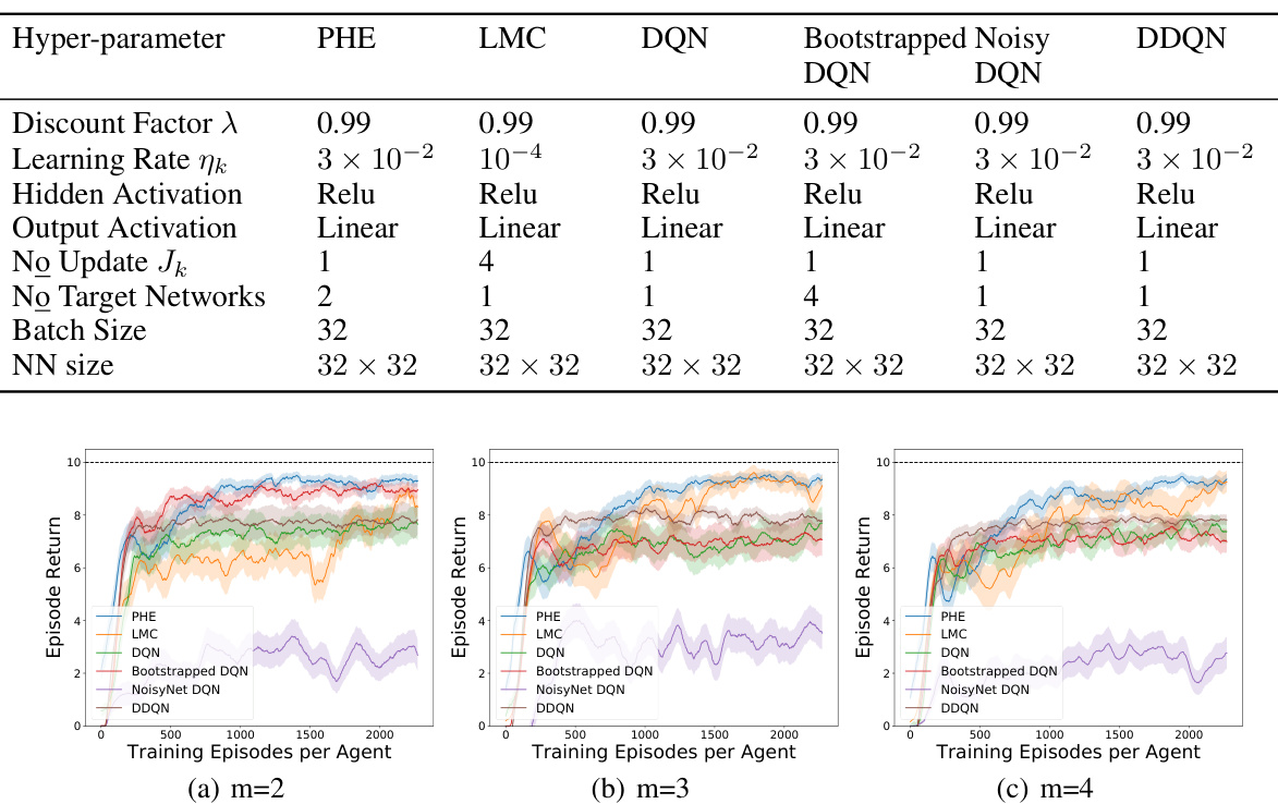
🔼 This figure compares the performance of different exploration strategies (PHE, LMC, DQN, Bootstrapped DQN, NoisyNet DQN, DDQN) across two different environments: N-chain and Super Mario Bros. The N-chain experiment uses a chain of 25 states, while the Super Mario Bros experiment uses a parallel setting. The results are averaged over 10 runs, with shaded areas representing standard deviations. The plots show episode return over training episodes per agent.
read the caption
Figure 1: Comparison among different exploration strategies in different environments. (a)-(b): N-chain with N = 25. (c)-(d): Super Mario Bros. All results are averaged over 10 runs and the shaded area represents the standard deviation.
🔼 This figure compares the performance of different exploration strategies (PHE, LMC, DQN, Bootstrapped DQN, NoisyNet DQN, DDQN) across two different environments: N-chain and Super Mario Bros. The N-chain environment is a simple, deep exploration problem with 25 states. Super Mario Bros is a more complex, partially observable environment. For both environments, the plot shows the average episode return for each algorithm across 10 independent runs, with shaded areas representing the standard deviation of the results. The figure demonstrates how different exploration strategies affect performance, particularly under conditions where exploration is challenging.
read the caption
Figure 1: Comparison among different exploration strategies in different environments. (a)-(b): N-chain with N = 25. (c)-(d): Super Mario Bros. All results are averaged over 10 runs and the shaded area represents the standard deviation.

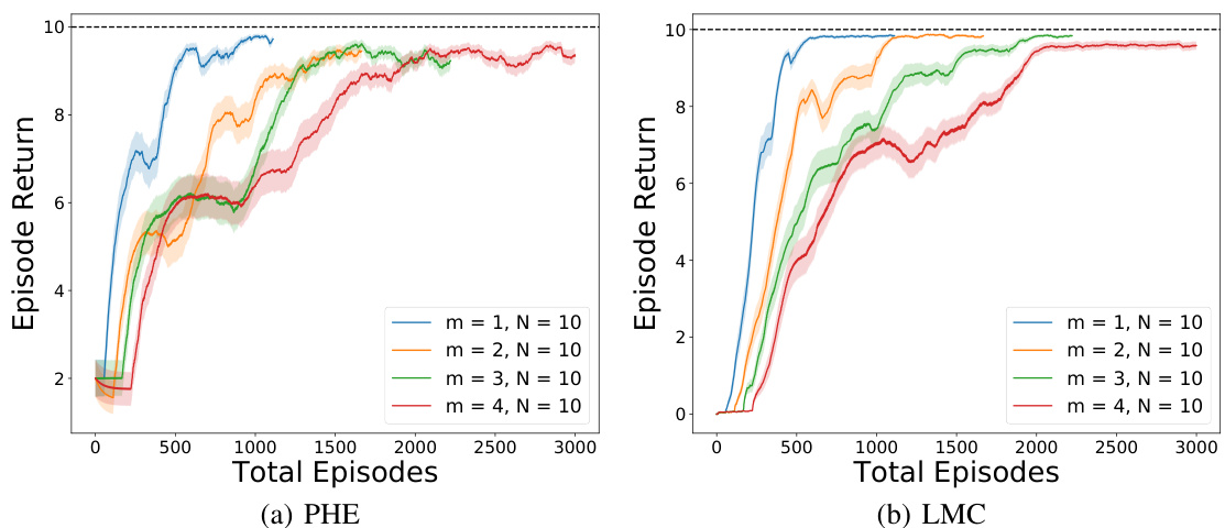
🔼 This figure compares the performance of PHE and LMC algorithms under different synchronization strategies (constant, exponential, and linear) and different numbers of agents (m=2,3,4) in a N-chain environment with N=10. It also shows results for single-agent and no-communication settings as baselines. The top row displays results for the PHE algorithm, while the bottom row shows results for the LMC algorithm. Each subplot shows episode return over total episodes, highlighting the impact of communication and different synchronization approaches on learning performance. The results indicate that, while centralized learning remains superior, various communication strategies substantially improve performance compared to no communication.
read the caption
Figure 6: Different number of agents m with different synchronization strategies as well as the single-agent and no communication settings in N = 10. Top: PHE, Bottom: LMC

🔼 This figure compares the performance of different exploration strategies (CoopTS-PHE, CoopTS-LMC, DQN, Double DQN, Bootstrapped DQN, and NoisyNet DQN) in two different environments: N-chain and Super Mario Bros. The N-chain results (a, b) show performance for different numbers of agents (m=2, m=3). The Super Mario Bros results (c, d) show performance with parallel and federated learning respectively. The shaded areas represent standard deviation. Overall, the CoopTS algorithms generally outperform the DQN baselines.
read the caption
Figure 1: Comparison among different exploration strategies in different environments. (a)-(b): N-chain with N = 25. (c)-(d): Super Mario Bros. All results are averaged over 10 runs and the shaded area represents the standard deviation.

🔼 The figure shows the computation time of different exploration strategies (PHE, LMC, DQN, Bootstrapped DQN, NoisyNet DQN, DDQN, NeuralTS, and NeuralUCB) with varying neural network sizes (32_2, 32_3, 64_2, and 64_3). The results indicate that PHE and LMC have relatively lower computation times compared to NeuralTS and NeuralUCB, especially as the neural network size increases.
read the caption
Figure 8: Computation time with different exploration strategies.
🔼 This figure compares the performance of different exploration strategies (PHE, LMC, DQN, Bootstrapped DQN, NoisyNet DQN, DDQN) across various multi-agent reinforcement learning environments. Subfigures (a) and (b) show results for the N-chain problem with 25 states, while subfigures (c) and (d) present results for the Super Mario Bros environment. Each result is an average of 10 independent runs, and shaded areas indicate standard deviation.
read the caption
Figure 1: Comparison among different exploration strategies in different environments. (a)-(b): N-chain with N = 25. (c)-(d): Super Mario Bros. All results are averaged over 10 runs and the shaded area represents the standard deviation.

🔼 This figure compares the performance of different exploration strategies (PHE, LMC, DQN, Bootstrapped DQN, NoisyNet DQN, and DDQN) across two different environments: N-chain and Super Mario Bros. The N-chain results show the average episode return for 2 and 3 agents over a varying number of training episodes. The Super Mario Bros. results show average episode return for the parallel and federated settings. In all cases, the shaded area represents the standard deviation across 10 independent runs, providing a visual representation of performance consistency. The figure demonstrates the effectiveness of the proposed randomized exploration strategies.
read the caption
Figure 1: Comparison among different exploration strategies in different environments. (a)-(b): N-chain with N = 25. (c)-(d): Super Mario Bros. All results are averaged over 10 runs and the shaded area represents the standard deviation.
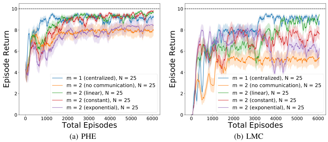
🔼 This figure compares the performance of different exploration strategies (PHE, LMC, DQN, Bootstrapped DQN, NoisyNet DQN, DDQN) across two different environments: N-chain and Super Mario Bros. The N-chain results (a and b) show the average episode return for 2 and 3 agents respectively, over 2000 training episodes. The Super Mario Bros results (c and d) show the performance of parallel and federated learning across 2000 training episodes. Shaded areas represent standard deviations, indicating the consistency of the results. The figure demonstrates that the proposed randomized exploration strategies (PHE and LMC) generally outperform the existing deep Q-network baselines, particularly in the N-chain deep exploration task.
read the caption
Figure 1: Comparison among different exploration strategies in different environments. (a)-(b): N-chain with N = 25. (c)-(d): Super Mario Bros. All results are averaged over 10 runs and the shaded area represents the standard deviation.
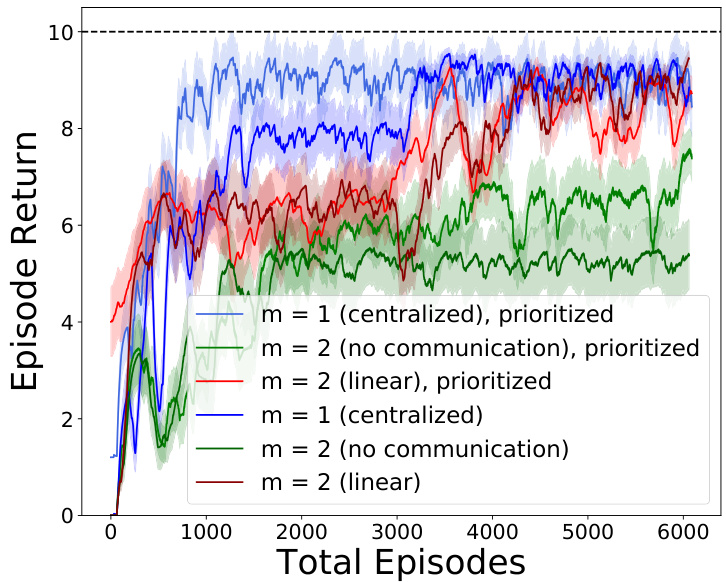
🔼 This figure compares the performance of different multi-agent reinforcement learning methods with and without prioritized experience replay in a parallel learning setting without inter-agent communication. The x-axis represents the total number of training episodes across all agents. The y-axis shows the average episode return. The results demonstrate that using prioritized experience replay can improve the learning performance, reducing the gap between centralized and parallel settings. The lines with similar colors represent the same settings with standard and prioritized experience replay, facilitating comparison of the performance improvement.
read the caption
Figure 12: Gap reduction improvement with prioritized experience replay for parallel learning without communication. Note that the same settings with standard and prioritized experience replay are in the same-ish color.

🔼 The figure compares the performance of different exploration strategies (PHE, LMC, DQN, Bootstrapped DQN, NoisyNet DQN, DDQN) in two different environments: N-chain and Super Mario Bros. The N-chain results show the average episode return for 2 and 3 agents, demonstrating the effectiveness of the proposed PHE and LMC methods. The Super Mario Bros results showcase the performance in parallel and federated learning settings. All results are averages over 10 runs, with shaded areas representing standard deviations.
read the caption
Figure 1: Comparison among different exploration strategies in different environments. (a)-(b): N-chain with N = 25. (c)-(d): Super Mario Bros. All results are averaged over 10 runs and the shaded area represents the standard deviation.

🔼 This figure compares the performance of various reinforcement learning algorithms (PHE, LMC, DQN, Bootstrapped DQN, NoisyNet DQN, DDQN) on a building energy system control task across four different cities with varying weather conditions (Tampa - hot humid, Tucson - hot dry, Rochester - cold humid, Great Falls - cold dry). The y-axis represents the daily return, which is a measure of the algorithm’s performance in terms of minimizing energy consumption while meeting temperature specifications. The x-axis represents the different algorithms. Violin plots are used to show the distribution of the daily return for each algorithm across multiple runs. The figure demonstrates the performance of the proposed randomized exploration strategies (PHE, LMC) compared to other baselines, showcasing their robustness across diverse environmental settings. Note that some algorithms (DQN, NoisyNet) perform poorly, suggesting that the discrete action space makes learning harder in this environment.
read the caption
Figure 14: Evaluation performance at different cities in building energy systems
More on tables

🔼 This table compares various single-agent and multi-agent reinforcement learning algorithms on episodic, non-stationary, linear Markov Decision Processes (MDPs). It shows the theoretical regret bounds (cumulative and average), whether the algorithm uses randomized exploration, whether it’s generalizable to deep RL, and its communication complexity. The table helps illustrate the efficiency and scalability of the proposed CoopTS-PHE and CoopTS-LMC algorithms compared to existing methods.
read the caption
Table 1: Comparison on episodic, non-stationary, linear MDPs. We define the average regret as the cumulative regret divided by the total number of samples (transition pairs) used by the algorithm. Here d is the feature dimension, H is the episode length, K is the number of episodes, and M is the number of agents in a multi-agent setting.

🔼 This table compares various algorithms (including the authors’ proposed CoopTS-PHE and CoopTS-LMC) on episodic, non-stationary, linear Markov Decision Processes (MDPs). It shows the theoretical regret and average regret bounds for each algorithm, along with whether they use randomized exploration and whether they are easily generalizable to deep reinforcement learning. It also lists the communication complexity for multi-agent settings. The table helps to highlight the performance and efficiency of the proposed methods in comparison to existing approaches.
read the caption
Table 1: Comparison on episodic, non-stationary, linear MDPs. We define the average regret as the cumulative regret divided by the total number of samples (transition pairs) used by the algorithm. Here d is the feature dimension, H is the episode length, K is the number of episodes, and M is the number of agents in a multi-agent setting.

🔼 This table compares different algorithms for episodic, non-stationary, linear Markov Decision Processes (MDPs). It shows the theoretical regret and average regret bounds for each algorithm, along with its communication complexity and whether it supports randomized exploration and generalizes to deep RL. The algorithms are categorized by whether they are for single-agent or multi-agent settings. The table highlights the proposed CoopTS-PHE and CoopTS-LMC algorithms, showing their superior performance in communication efficiency and regret bounds.
read the caption
Table 1: Comparison on episodic, non-stationary, linear MDPs. We define the average regret as the cumulative regret divided by the total number of samples (transition pairs) used by the algorithm. Here d is the feature dimension, H is the episode length, K is the number of episodes, and M is the number of agents in a multi-agent setting.
🔼 This table compares the performance of various algorithms (including the authors’ proposed methods) on episodic, non-stationary, linear Markov Decision Processes (MDPs). It shows the theoretical regret and average regret bounds for each algorithm, along with whether they incorporate randomized exploration and are generalizable to deep reinforcement learning. It also provides the communication complexity for multi-agent settings.
read the caption
Table 1: Comparison on episodic, non-stationary, linear MDPs. We define the average regret as the cumulative regret divided by the total number of samples (transition pairs) used by the algorithm. Here d is the feature dimension, H is the episode length, K is the number of episodes, and M is the number of agents in a multi-agent setting.

🔼 This table compares the performance of different algorithms on episodic, non-stationary, linear Markov Decision Processes (MDPs). It shows the theoretical regret bound, average regret, whether the algorithm uses randomized exploration, if it is generalizable to deep reinforcement learning, and the communication complexity for each algorithm. The algorithms are categorized into single-agent and multi-agent settings, and the table highlights the proposed CoopTS-PHE and CoopTS-LMC algorithms alongside existing methods.
read the caption
Table 1: Comparison on episodic, non-stationary, linear MDPs. We define the average regret as the cumulative regret divided by the total number of samples (transition pairs) used by the algorithm. Here d is the feature dimension, H is the episode length, K is the number of episodes, and M is the number of agents in a multi-agent setting.
Full paper#


