TL;DR#
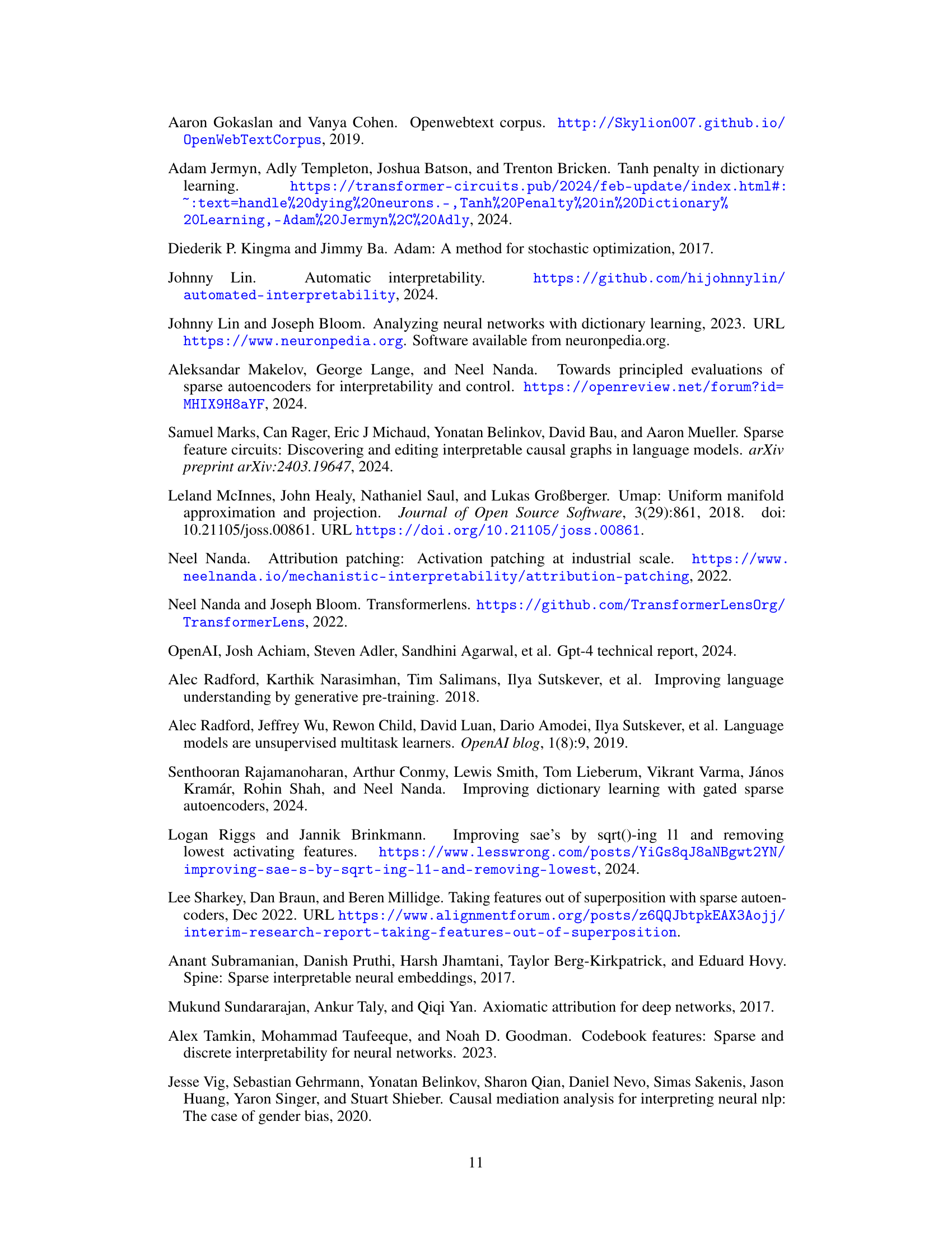
Understanding how neural networks function is a major challenge in AI. Sparse autoencoders (SAEs) have been used to identify the network’s features by learning a sparse dictionary that reconstructs the network’s internal activations; however, these SAEs may focus more on dataset structure than the network’s computational structure. Existing SAEs suffer from feature splitting and feature suppression, hindering accurate feature identification.
This paper introduces a novel method: end-to-end (e2e) SAE training. Instead of minimizing reconstruction error, e2e SAEs minimize the KL divergence between the output distributions of the original model and the model with SAE activations inserted. This approach ensures that the learned features are functionally important. Results show that e2e SAEs require fewer features, achieve better performance, and maintain high interpretability compared to standard SAEs, representing a Pareto improvement. The authors also provide a library and resources to facilitate reproducibility.
Key Takeaways#
Why does it matter?#
This paper significantly advances mechanistic interpretability by introducing end-to-end sparse autoencoders. It offers a more efficient and accurate way to identify functionally important features in neural networks, opening new avenues for research and impacting various fields.
Visual Insights#

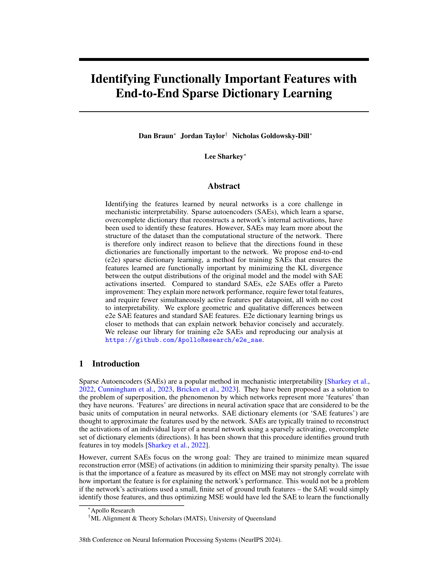
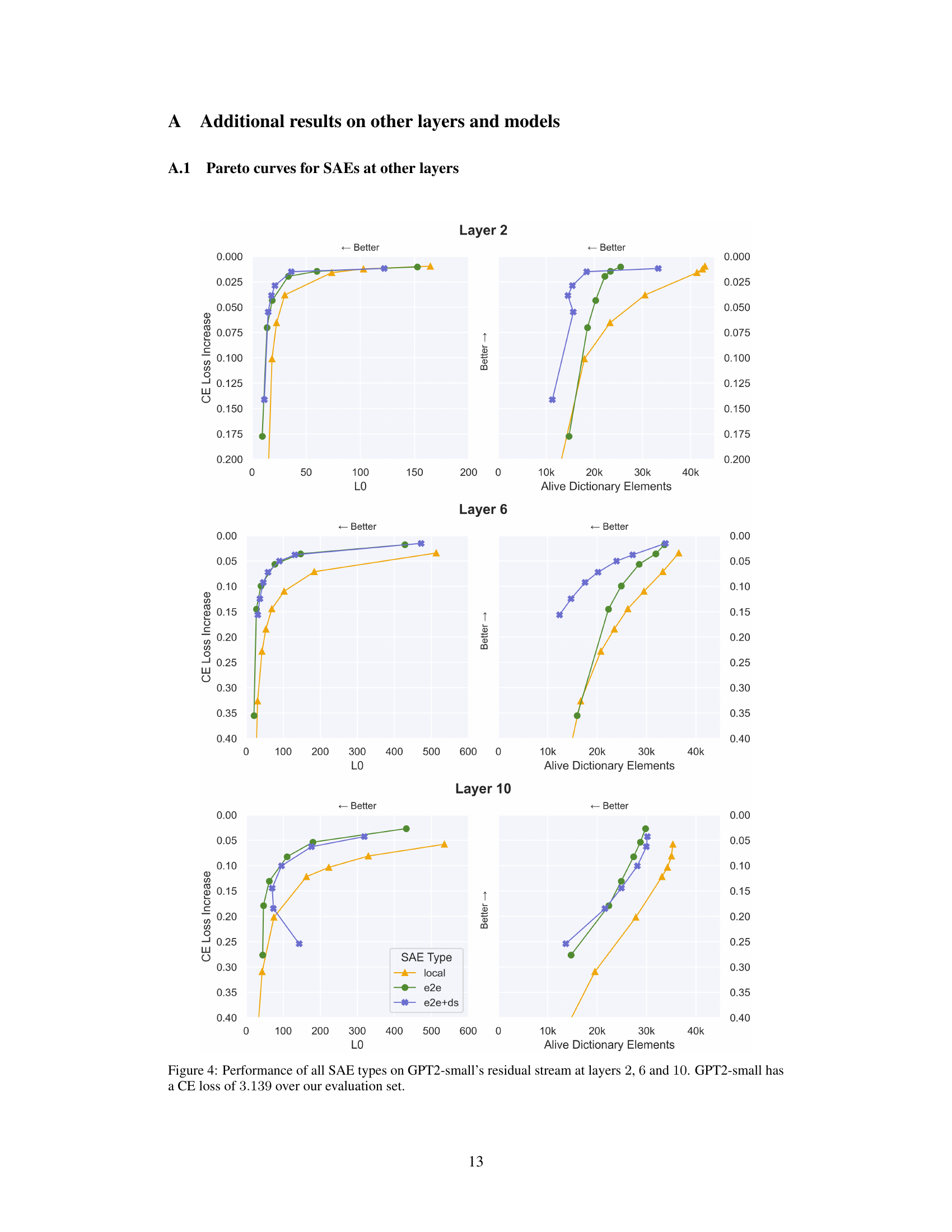
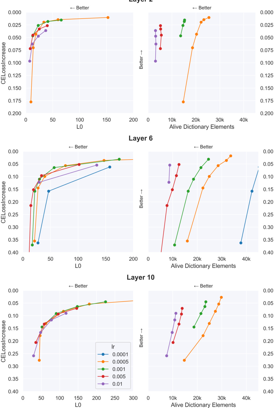
🔼 The figure compares three types of sparse autoencoders (SAEs) for training: SAElocal, SAEe2e, and SAEe2e+ds. The top panel is a diagram illustrating the different loss functions used for each SAE type. SAElocal uses mean squared error (MSE) to reconstruct the original activations. SAEe2e uses Kullback-Leibler (KL) divergence between the original model’s output distribution and the model’s output distribution with SAE activations inserted. SAEe2e+ds adds MSE reconstruction loss at downstream layers to the KL divergence loss. All three SAE types include an L1 sparsity penalty. The bottom panel shows Pareto curves illustrating the trade-off between the number of features and cross-entropy (CE) loss increase for each SAE type on GPT2-small layer 6. The e2e SAEs (SAEe2e and SAEe2e+ds) achieve better performance (lower CE loss increase) with fewer features compared to SAElocal.
read the caption
Figure 1: Top: Diagram comparing the loss terms used to train each type of SAE. Each arrow is a loss term which compares the activations represented by circles. SAElocal uses MSE reconstruction loss between the SAE input and the SAE output. SAEe2e uses KL-divergence on the logits. SAEe2e+ds (end-to-end + downstream reconstruction) uses KL-divergence in addition to the sum of the MSE reconstruction losses at all future layers. All three are additionally trained with a L₁ sparsity penalty (not pictured). Bottom: Pareto curves for three different types of GPT2-small layer 6 SAEs as the sparsity coefficient is varied. E2e-SAEs require fewer features per datapoint (i.e. have a lower Lo) and fewer features over the entire dataset (i.e. have a low number of alive dictionary elements). GPT2-small has a CE loss of 3.139 over our evaluation set.

🔼 This table compares three different types of Sparse Autoencoders (SAEs) trained on layer 6 of a GPT2-small model. The SAEs are designed to identify functionally important features in the model. The table shows the sparsity coefficient (λ), the average number of active features per data point (Lo), the total number of active dictionary elements, and the increase in cross-entropy loss (CE Loss Increase) for each SAE type. The comparison focuses on SAEs with approximately equivalent CE loss increases to highlight differences in other metrics.
read the caption
Table 1: Three SAEs from layer 6 with similar CE loss increases are analyzed in detail.
In-depth insights#
End-to-End SAEs#
The core concept of “End-to-End SAEs” revolves around directly optimizing sparse autoencoders (SAEs) to enhance the network’s overall performance, instead of merely focusing on reconstructing intermediate layer activations. This end-to-end approach minimizes the Kullback-Leibler (KL) divergence between the original model’s output distribution and that of the model using SAE-modified activations. By doing so, it ensures that the learned features are functionally important for the network’s primary task, rather than simply capturing dataset structure. This results in Pareto improvements: better explained variance with fewer, less active features, and improved feature orthogonality (less feature splitting). The method addresses previous limitations of standard SAEs, where features weren’t necessarily aligned with functional importance, by shifting the focus from reconstruction error minimization to optimizing a performance metric. The inclusion of downstream reconstruction loss further refines this process, ensuring the SAE’s output doesn’t disrupt the downstream layers’ computations.
Pareto Improvement#
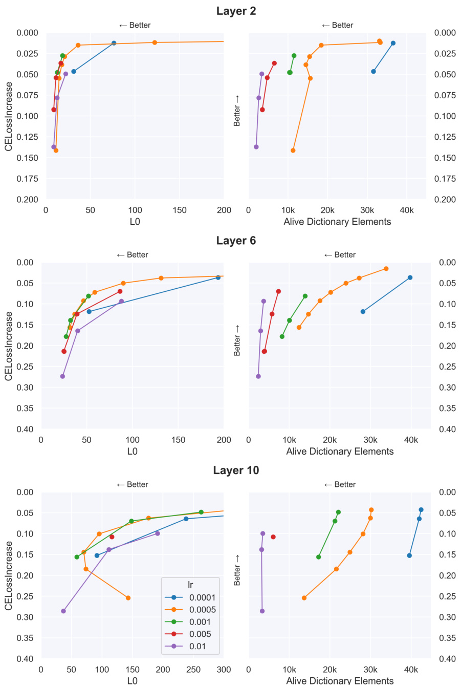
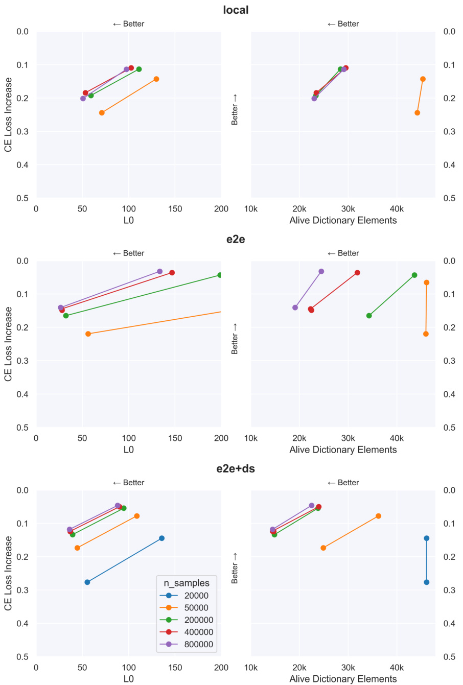
The concept of “Pareto improvement” in the context of the research paper signifies a situation where a model exhibits enhanced performance across multiple metrics without sacrificing performance in any single metric. End-to-end Sparse Autoencoders (e2e SAEs), as presented in the paper, achieve this Pareto improvement over standard SAEs by minimizing the KL divergence between the original model’s output and the model’s output when using SAE activations. This approach not only yields better explanation of network performance but also reduces the number of required features and the number of simultaneously active features, all without compromising interpretability. The e2e training method is key, leading to a more efficient and concise understanding of the network’s behavior. This improvement is significant because it addresses previous limitations of SAEs, such as feature splitting and a focus on MSE minimization that doesn’t directly translate to functional importance.
Feature Orthogonality#
The concept of feature orthogonality is crucial for understanding the quality of learned representations in sparse autoencoders (SAEs). Orthogonal features ideally represent independent aspects of the data, minimizing redundancy and improving the interpretability of the model. The paper investigates how different training methods for SAEs impact feature orthogonality. End-to-end trained SAEs demonstrate greater feature orthogonality compared to locally trained SAEs, suggesting that their features are more distinct and less prone to the phenomenon of ‘feature splitting’, where a single feature is unnecessarily divided into multiple similar ones. This higher orthogonality, achieved by focusing on the functional importance of features rather than reconstruction error, directly contributes to improved efficiency by requiring fewer features to explain the same amount of network performance. This is a significant finding because it shows that prioritizing functional importance during training naturally leads to a more interpretable and concise representation of the data, which is a key goal of mechanistic interpretability research.
Interpretability Tradeoffs#
The concept of ‘Interpretability Tradeoffs’ in the context of a research paper analyzing sparse autoencoders (SAEs) for neural network interpretability is multifaceted. It acknowledges that increasing the interpretability of a model, by using techniques such as SAEs to isolate and represent features, often comes at a cost. This cost is frequently manifested as a decrease in downstream task performance. The paper likely explores the balance between obtaining a concise, understandable representation of the model’s internal workings (high interpretability) and maintaining strong predictive accuracy on the tasks the model was originally trained for. The tradeoff might involve the size of the feature dictionary in SAEs: larger dictionaries could offer more granular explanations but also lead to increased computational costs and potentially overfitting, reducing generalization. Similarly, stricter sparsity constraints in SAE training can enhance interpretability by limiting the number of simultaneously active features, but may sacrifice the richness of representation, thus impacting performance. A key insight explored would be the Pareto efficiency frontier, identifying those configurations where improvements in interpretability are not achieved at the cost of performance. The paper’s analysis likely highlights the need to find an optimal balance depending on the specific application and its prioritization of interpretability versus performance.
Future Work#
Future research directions stemming from this paper could explore several promising avenues. Extending the end-to-end SAE framework to other model architectures and datasets is crucial to establish generalizability. Investigating the impact of different sparsity penalties and architectural modifications on performance and interpretability would further enhance the method’s efficacy. A deeper dive into the qualitative analysis of learned features, potentially through advanced visualization techniques and larger-scale human evaluation, could uncover valuable insights into the functional roles of these features and the underlying mechanisms of the model. Finally, applying e2e SAEs to diverse downstream tasks, including those beyond simple prediction, would allow researchers to explore the method’s capabilities across a broader spectrum of applications and advance mechanistic interpretability beyond its current limitations.
More visual insights#
More on figures
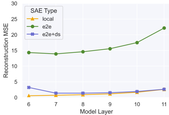
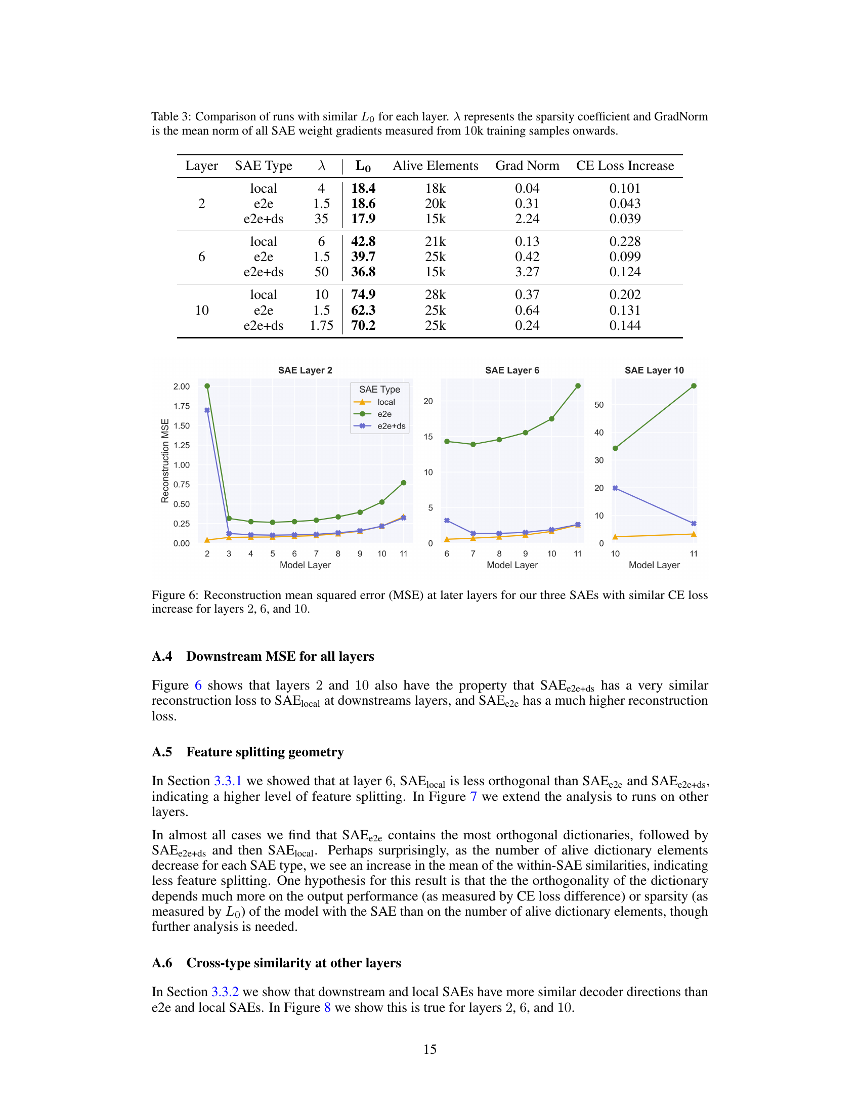
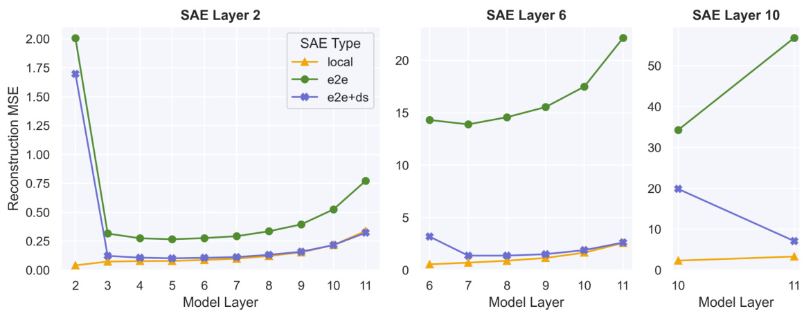
🔼 This figure compares the reconstruction mean squared error (MSE) at different layers in a model for three different types of sparse autoencoders (SAEs): SAElocal, SAEe2e, and SAEe2e+ds. The SAEs were trained on GPT2-small layer 6 and selected to have similar cross-entropy loss increases. SAElocal focuses on minimizing MSE at layer 6. SAEe2e matches the output probability distribution. SAEe2e+ds matches the output probability distribution and minimizes MSE in subsequent layers. The graph shows that SAElocal has the lowest MSE at layer 6 but significantly higher MSE in later layers. SAEe2e and SAEe2e+ds exhibit greater MSE throughout, but the differences between them are less pronounced.
read the caption
Figure 2: Reconstruction mean squared error (MSE) at later layers for our set of GPT2-small layer 6 SAEs with similar CE loss increases (Table 1). SAElocal is trained to minimize MSE at layer 6, SAEe2e was trained to match the output probability distribution, SAEe2e+ds was trained to match the output probability distribution and minimize MSE in all downstream layers.

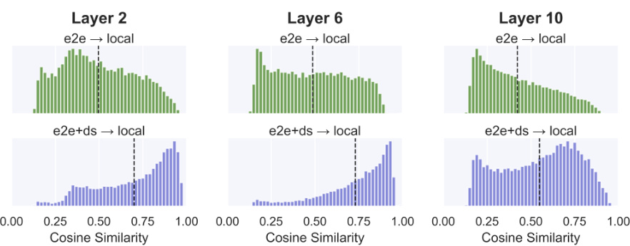
🔼 This figure presents a comparison of the geometric properties of features learned by three different types of Sparse Autoencoders (SAEs): local, e2e, and e2e+ds. The comparison is done for layer 6 of the GPT2-small model. Three subplots show the cosine similarity distributions: (a) within the same SAE type, showing the similarity between features within a given SAE; (b) across different random seeds for the same SAE type, indicating the robustness of the features to different random initializations; and (c) between different SAE types (comparing e2e and e2e+ds to local), illustrating the similarity of features learned by different training methods. The results show differences in feature clustering and similarity across different SAEs, highlighting the impact of the training method on the learned feature representations.
read the caption
Figure 3: Geometric comparisons for our set of GPT2-small layer 6 SAEs with similar CE loss increases (Table 1). For each dictionary element, we find the max cosine similarity between itself and all other dictionary elements. In 3a we compare to others directions in the same SAE, in 3b to directions in an SAE of the same type trained with a different random seed, in 3c to directions in the SAElocal with similar CE loss increase.

🔼 The figure compares three different methods for training Sparse Autoencoders (SAEs): SAElocal, SAEe2e, and SAEe2e+ds. The top panel shows a diagram illustrating the loss functions used for each method. SAElocal uses mean squared error (MSE) to reconstruct the input activations. SAEe2e uses Kullback-Leibler (KL) divergence to ensure the output distribution of the model with the SAE inserted matches the original model. SAEe2e+ds adds MSE reconstruction losses at all subsequent layers to further ensure faithfulness. The bottom panel shows Pareto curves comparing the three methods. The curves plot the cross-entropy (CE) loss increase versus the number of features used. The end-to-end methods (SAEe2e and SAEe2e+ds) are shown to achieve a Pareto improvement over SAElocal, needing fewer features to achieve similar performance.
read the caption
Figure 1: Top: Diagram comparing the loss terms used to train each type of SAE. Each arrow is a loss term which compares the activations represented by circles. SAElocal uses MSE reconstruction loss between the SAE input and the SAE output. SAEe2e uses KL-divergence on the logits. SAEe2e+ds (end-to-end + downstream reconstruction) uses KL-divergence in addition to the sum of the MSE reconstruction losses at all future layers. All three are additionally trained with a L₁ sparsity penalty (not pictured). Bottom: Pareto curves for three different types of GPT2-small layer 6 SAEs as the sparsity coefficient is varied. E2e-SAEs require fewer features per datapoint (i.e. have a lower Lo) and fewer features over the entire dataset (i.e. have a low number of alive dictionary elements). GPT2-small has a CE loss of 3.139 over our evaluation set.

🔼 The figure compares three different methods for training sparse autoencoders (SAEs): SAElocal, SAEe2e, and SAEe2e+ds. The top panel shows a diagram illustrating the different loss functions used in each method. SAElocal uses mean squared error (MSE) to reconstruct the input activations. SAEe2e uses Kullback-Leibler (KL) divergence to minimize the difference between the output distributions of the original model and the model with SAE activations inserted. SAEe2e+ds adds an additional MSE loss term for downstream layers. All three methods also use an L1 sparsity penalty. The bottom panel shows Pareto curves for the three SAE types, demonstrating that end-to-end SAEs (SAEe2e and SAEe2e+ds) require fewer features to explain the same amount of network performance compared to SAElocal.
read the caption
Figure 1: Top: Diagram comparing the loss terms used to train each type of SAE. Each arrow is a loss term which compares the activations represented by circles. SAElocal uses MSE reconstruction loss between the SAE input and the SAE output. SAEe2e uses KL-divergence on the logits. SAEe2e+ds (end-to-end + downstream reconstruction) uses KL-divergence in addition to the sum of the MSE reconstruction losses at all future layers. All three are additionally trained with a L₁ sparsity penalty (not pictured). Bottom: Pareto curves for three different types of GPT2-small layer 6 SAEs as the sparsity coefficient is varied. E2e-SAEs require fewer features per datapoint (i.e. have a lower Lo) and fewer features over the entire dataset (i.e. have a low number of alive dictionary elements). GPT2-small has a CE loss of 3.139 over our evaluation set.
🔼 The figure compares the reconstruction mean squared error (MSE) at different layers for three types of Sparse Autoencoders (SAEs) trained on layer 6 of GPT2-small. The SAEs have similar cross-entropy (CE) loss increases. The SAElocal model focuses on minimizing MSE at layer 6. The SAEe2e model aims to match the output probability distribution. The SAEe2e+ds model aims to match both the output probability distribution and minimize MSE in subsequent layers. The plot shows that SAElocal has the lowest MSE at layer 6, as expected, because it is trained to minimize it there. However, SAElocal’s MSE increases dramatically in later layers. SAEe2e and SAEe2e+ds exhibit relatively stable MSE across the layers, indicating that they are better at generalizing beyond layer 6.
read the caption
Figure 2: Reconstruction mean squared error (MSE) at later layers for our set of GPT2-small layer 6 SAEs with similar CE loss increases (Table 1). SAElocal is trained to minimize MSE at layer 6, SAEe2e was trained to match the output probability distribution, SAEe2e+ds was trained to match the output probability distribution and minimize MSE in all downstream layers.

🔼 The figure compares three different types of sparse autoencoders (SAEs): SAElocal, SAEe2e, and SAEe2e+ds. The top panel is a diagram illustrating the loss functions used to train each SAE type. The bottom panel shows Pareto curves illustrating the trade-off between the number of features used and the performance (measured by cross-entropy loss increase) for each SAE type on a GPT2-small model. The key finding is that end-to-end SAEs (SAEe2e and SAEe2e+ds) achieve better performance with fewer features than SAElocal.
read the caption
Figure 1: Top: Diagram comparing the loss terms used to train each type of SAE. Each arrow is a loss term which compares the activations represented by circles. SAElocal uses MSE reconstruction loss between the SAE input and the SAE output. SAEe2e uses KL-divergence on the logits. SAEe2e+ds (end-to-end + downstream reconstruction) uses KL-divergence in addition to the sum of the MSE reconstruction losses at all future layers. All three are additionally trained with a L₁ sparsity penalty (not pictured). Bottom: Pareto curves for three different types of GPT2-small layer 6 SAEs as the sparsity coefficient is varied. E2e-SAEs require fewer features per datapoint (i.e. have a lower Lo) and fewer features over the entire dataset (i.e. have a low number of alive dictionary elements). GPT2-small has a CE loss of 3.139 over our evaluation set.
🔼 This figure compares the geometric properties of features learned by three different types of Sparse Autoencoders (SAEs): SAElocal, SAEe2e, and SAEe2e+ds. Subfigure 3a shows the within-SAE cosine similarity, indicating feature splitting and clustering. Subfigure 3b shows the similarity of features across different random seeds, evaluating the robustness of the models. Subfigure 3c compares the similarity between SAEe2e and SAEe2e+ds features to those of SAElocal, illustrating differences in feature geometry between methods.
read the caption
Figure 3: Geometric comparisons for our set of GPT2-small layer 6 SAEs with similar CE loss increases (Table 1). For each dictionary element, we find the max cosine similarity between itself and all other dictionary elements. In 3a we compare to others directions in the same SAE, in 3b to directions in an SAE of the same type trained with a different random seed, in 3c to directions in the SAElocal with similar CE loss increase.

🔼 The figure compares the reconstruction error (MSE) at different layers after inserting three different types of Sparse Autoencoders (SAEs): SAElocal, SAEe2e, and SAEe2e+ds. SAElocal is trained to minimize MSE at layer 6. SAEe2e is trained to match the output probability distribution using KL divergence, and SAEe2e+ds incorporates both KL divergence and MSE loss in downstream layers. The graph shows that while SAElocal achieves low MSE at layer 6 (as expected due to its training objective), the reconstruction error of SAEe2e and SAEe2e+ds significantly increase in the downstream layers, highlighting their different training objectives and effects on the network’s computations.
read the caption
Figure 2: Reconstruction mean squared error (MSE) at later layers for our set of GPT2-small layer 6 SAEs with similar CE loss increases (Table 1). SAElocal is trained to minimize MSE at layer 6, SAEe2e was trained to match the output probability distribution, SAEe2e+ds was trained to match the output probability distribution and minimize MSE in all downstream layers.

🔼 The top part of the figure shows a diagram that compares the loss terms used for training three different types of Sparse Autoencoders (SAEs): SAElocal, SAEe2e, and SAEe2e+ds. Each loss term is represented by an arrow connecting circles representing the activations at different points in the network. The bottom part shows Pareto curves for the three SAE types, illustrating the trade-off between the number of features used and the cross-entropy (CE) loss increase. The Pareto curves demonstrate that end-to-end SAEs (e2e SAEs) achieve better performance (lower CE loss) with fewer features, both per data point (lower Lo) and across the entire dataset (fewer alive dictionary elements).
read the caption
Figure 1: Top: Diagram comparing the loss terms used to train each type of SAE. Each arrow is a loss term which compares the activations represented by circles. SAElocal uses MSE reconstruction loss between the SAE input and the SAE output. SAEe2e uses KL-divergence on the logits. SAEe2e+ds (end-to-end + downstream reconstruction) uses KL-divergence in addition to the sum of the MSE reconstruction losses at all future layers. All three are additionally trained with a L₁ sparsity penalty (not pictured). Bottom: Pareto curves for three different types of GPT2-small layer 6 SAEs as the sparsity coefficient is varied. E2e-SAEs require fewer features per datapoint (i.e. have a lower Lo) and fewer features over the entire dataset (i.e. have a low number of alive dictionary elements). GPT2-small has a CE loss of 3.139 over our evaluation set.

🔼 The figure shows a comparison of three different types of sparse autoencoders (SAEs): SAElocal, SAEe2e, and SAEe2e+ds. The top panel is a diagram illustrating the different loss functions used to train each SAE type. SAElocal uses mean squared error (MSE) to reconstruct the input activations. SAEe2e uses Kullback-Leibler (KL) divergence between the output distributions of the original model and the model with SAE activations. SAEe2e+ds combines KL divergence with MSE reconstruction losses at downstream layers. All three are trained with an L1 sparsity penalty. The bottom panel shows Pareto curves comparing the performance (CE loss) and efficiency (number of features) of the three SAE types on GPT2-small layer 6. The curves demonstrate that e2e SAEs (SAEe2e and SAEe2e+ds) achieve better performance with fewer features than SAElocal.
read the caption
Figure 1: Top: Diagram comparing the loss terms used to train each type of SAE. Each arrow is a loss term which compares the activations represented by circles. SAElocal uses MSE reconstruction loss between the SAE input and the SAE output. SAEe2e uses KL-divergence on the logits. SAEe2e+ds (end-to-end + downstream reconstruction) uses KL-divergence in addition to the sum of the MSE reconstruction losses at all future layers. All three are additionally trained with a L1 sparsity penalty (not pictured). Bottom: Pareto curves for three different types of GPT2-small layer 6 SAEs as the sparsity coefficient is varied. E2e-SAEs require fewer features per datapoint (i.e. have a lower L0) and fewer features over the entire dataset (i.e. have a low number of alive dictionary elements). GPT2-small has a CE loss of 3.139 over our evaluation set.

🔼 This figure compares three different methods for training Sparse Autoencoders (SAEs): SAElocal, SAEe2e, and SAEe2e+ds. The top panel is a diagram illustrating the loss functions used in each method. SAElocal minimizes the mean squared error (MSE) between the input and output activations of the SAE. SAEe2e minimizes the Kullback-Leibler (KL) divergence between the output distributions of the original model and the model with SAE activations inserted. SAEe2e+ds combines the KL divergence with the MSE reconstruction losses at all subsequent layers. All three methods also include a sparsity penalty. The bottom panel shows Pareto curves comparing the three SAE training methods across different sparsity levels. The curves plot the cross-entropy (CE) loss increase against the number of active dictionary elements (alive dictionary elements) and Lo (average number of features activated per data point). The results show that SAEe2e and SAEe2e+ds achieve a Pareto improvement over SAElocal, requiring fewer features to explain the same amount of network performance.
read the caption
Figure 1: Top: Diagram comparing the loss terms used to train each type of SAE. Each arrow is a loss term which compares the activations represented by circles. SAElocal uses MSE reconstruction loss between the SAE input and the SAE output. SAEe2e uses KL-divergence on the logits. SAEe2e+ds (end-to-end + downstream reconstruction) uses KL-divergence in addition to the sum of the MSE reconstruction losses at all future layers. All three are additionally trained with a L₁ sparsity penalty (not pictured). Bottom: Pareto curves for three different types of GPT2-small layer 6 SAEs as the sparsity coefficient is varied. E2e-SAEs require fewer features per datapoint (i.e. have a lower Lo) and fewer features over the entire dataset (i.e. have a low number of alive dictionary elements). GPT2-small has a CE loss of 3.139 over our evaluation set.
🔼 The figure demonstrates the training process and performance comparison of three different types of Sparse Autoencoders (SAEs): SAElocal, SAEe2e, and SAEe2e+ds. The top panel illustrates the different loss terms used for training each SAE type, showing how SAElocal focuses solely on reconstructing the input activations, while SAEe2e and SAEe2e+ds incorporate KL divergence to ensure functional importance of the learned features. The bottom panel presents Pareto curves, showing the trade-off between the number of features and the cross-entropy loss increase. The results highlight the Pareto improvement achieved by e2e SAEs (SAEe2e and SAEe2e+ds), requiring fewer features for the same level of performance improvement compared to SAElocal.
read the caption
Figure 1: Top: Diagram comparing the loss terms used to train each type of SAE. Each arrow is a loss term which compares the activations represented by circles. SAElocal uses MSE reconstruction loss between the SAE input and the SAE output. SAEe2e uses KL-divergence on the logits. SAEe2e+ds (end-to-end + downstream reconstruction) uses KL-divergence in addition to the sum of the MSE reconstruction losses at all future layers. All three are additionally trained with a L₁ sparsity penalty (not pictured). Bottom: Pareto curves for three different types of GPT2-small layer 6 SAEs as the sparsity coefficient is varied. E2e-SAEs require fewer features per datapoint (i.e. have a lower Lo) and fewer features over the entire dataset (i.e. have a low number of alive dictionary elements). GPT2-small has a CE loss of 3.139 over our evaluation set.
🔼 The figure compares three different training methods for Sparse Autoencoders (SAEs): * SAElocal: Uses Mean Squared Error (MSE) to reconstruct the input activations. * SAEe2e: Uses Kullback-Leibler (KL) divergence between the original model’s output logits and the model’s output logits with SAE activations inserted. * SAEe2e+ds: Combines KL divergence with MSE reconstruction losses at subsequent layers. The top part illustrates the loss functions used in each method, showing the relationships between the input, SAE, and output activations. The bottom part shows Pareto curves comparing the three methods across different sparsity levels, demonstrating the Pareto improvement offered by the e2e SAEs. E2e SAEs require fewer total features and features per datapoint to explain the same level of network performance, without compromising interpretability.
read the caption
Figure 1: Top: Diagram comparing the loss terms used to train each type of SAE. Each arrow is a loss term which compares the activations represented by circles. SAElocal uses MSE reconstruction loss between the SAE input and the SAE output. SAEe2e uses KL-divergence on the logits. SAEe2e+ds (end-to-end + downstream reconstruction) uses KL-divergence in addition to the sum of the MSE reconstruction losses at all future layers. All three are additionally trained with a L₁ sparsity penalty (not pictured). Bottom: Pareto curves for three different types of GPT2-small layer 6 SAEs as the sparsity coefficient is varied. E2e-SAEs require fewer features per datapoint (i.e. have a lower Lo) and fewer features over the entire dataset (i.e. have a low number of alive dictionary elements). GPT2-small has a CE loss of 3.139 over our evaluation set.

🔼 The figure compares three different methods for training sparse autoencoders (SAEs): SAElocal, SAEe2e, and SAEe2e+ds. The top panel shows a diagram illustrating the loss functions used in each method. SAElocal minimizes mean squared error (MSE) between the input and output activations of the SAE. SAEe2e minimizes the Kullback-Leibler (KL) divergence between the output logits of the original model and the model with the SAE’s activations inserted. SAEe2e+ds combines the KL divergence loss with additional MSE reconstruction losses at downstream layers. The bottom panel presents Pareto curves showing the trade-off between the number of features used and the cross-entropy (CE) loss increase when using the SAE’s activations. The curves demonstrate that e2e SAEs (SAEe2e and SAEe2e+ds) achieve better performance with fewer features compared to SAElocal.
read the caption
Figure 1: Top: Diagram comparing the loss terms used to train each type of SAE. Each arrow is a loss term which compares the activations represented by circles. SAElocal uses MSE reconstruction loss between the SAE input and the SAE output. SAEe2e uses KL-divergence on the logits. SAEe2e+ds (end-to-end + downstream reconstruction) uses KL-divergence in addition to the sum of the MSE reconstruction losses at all future layers. All three are additionally trained with a L₁ sparsity penalty (not pictured). Bottom: Pareto curves for three different types of GPT2-small layer 6 SAEs as the sparsity coefficient is varied. E2e-SAEs require fewer features per datapoint (i.e. have a lower Lo) and fewer features over the entire dataset (i.e. have a low number of alive dictionary elements). GPT2-small has a CE loss of 3.139 over our evaluation set.
🔼 The figure compares three different types of sparse autoencoders (SAEs): SAElocal, SAEe2e, and SAEe2e+ds. The top panel illustrates the loss functions used to train each SAE. SAElocal uses mean squared error (MSE) to reconstruct the input activations. SAEe2e uses Kullback-Leibler (KL) divergence to match the output distribution of the original model with the model using SAE activations. SAEe2e+ds combines KL divergence with MSE reconstruction losses from subsequent layers. All SAEs also include an L1 sparsity penalty. The bottom panel shows Pareto curves illustrating the trade-off between the number of features used and the cross-entropy (CE) loss increase. E2e SAEs (SAEe2e and SAEe2e+ds) achieve lower CE loss increase with fewer features compared to SAElocal, demonstrating Pareto improvement.
read the caption
Figure 1: Top: Diagram comparing the loss terms used to train each type of SAE. Each arrow is a loss term which compares the activations represented by circles. SAElocal uses MSE reconstruction loss between the SAE input and the SAE output. SAEe2e uses KL-divergence on the logits. SAEe2e+ds (end-to-end + downstream reconstruction) uses KL-divergence in addition to the sum of the MSE reconstruction losses at all future layers. All three are additionally trained with a L₁ sparsity penalty (not pictured). Bottom: Pareto curves for three different types of GPT2-small layer 6 SAEs as the sparsity coefficient is varied. E2e-SAEs require fewer features per datapoint (i.e. have a lower Lo) and fewer features over the entire dataset (i.e. have a low number of alive dictionary elements). GPT2-small has a CE loss of 3.139 over our evaluation set.

🔼 The figure compares three different methods for training sparse autoencoders (SAEs): SAElocal, SAEe2e, and SAEe2e+ds. The top panel shows a diagram illustrating the loss functions used in each method. SAElocal minimizes mean squared error (MSE) between the input and output activations. SAEe2e minimizes the Kullback-Leibler (KL) divergence between the output distributions of the original model and the model with SAE activations. SAEe2e+ds combines KL divergence with MSE reconstruction losses at downstream layers. All three methods include an L1 sparsity penalty. The bottom panel shows Pareto curves for the three SAE types, illustrating their trade-off between the number of features and cross-entropy (CE) loss increase. The e2e methods (SAEe2e and SAEe2e+ds) achieve a Pareto improvement, requiring fewer features for the same CE loss increase.
read the caption
Figure 1: Top: Diagram comparing the loss terms used to train each type of SAE. Each arrow is a loss term which compares the activations represented by circles. SAElocal uses MSE reconstruction loss between the SAE input and the SAE output. SAEe2e uses KL-divergence on the logits. SAEe2e+ds (end-to-end + downstream reconstruction) uses KL-divergence in addition to the sum of the MSE reconstruction losses at all future layers. All three are additionally trained with a L₁ sparsity penalty (not pictured). Bottom: Pareto curves for three different types of GPT2-small layer 6 SAEs as the sparsity coefficient is varied. E2e-SAEs require fewer features per datapoint (i.e. have a lower Lo) and fewer features over the entire dataset (i.e. have a low number of alive dictionary elements). GPT2-small has a CE loss of 3.139 over our evaluation set.
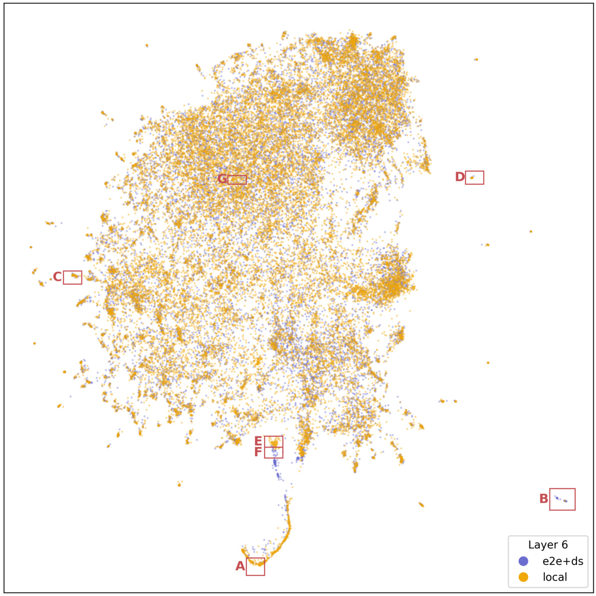
🔼 This UMAP plot visualizes the qualitative differences between the features learned by SAEe2e+ds and SAElocal for layer 6 of the GPT2-small model. The plot shows some distinct regions that are dense with SAEe2e+ds features but void of SAElocal features, and vice versa. These regions suggest qualitative differences in the types of features learned by each method. The plot is labeled with regions A through G, which are further described in the paper.
read the caption
Figure 19: UMAP plot of SAEe2e+ds and SAElocal features for layer 6 on runs with similar CE loss increase in GPT2-small.
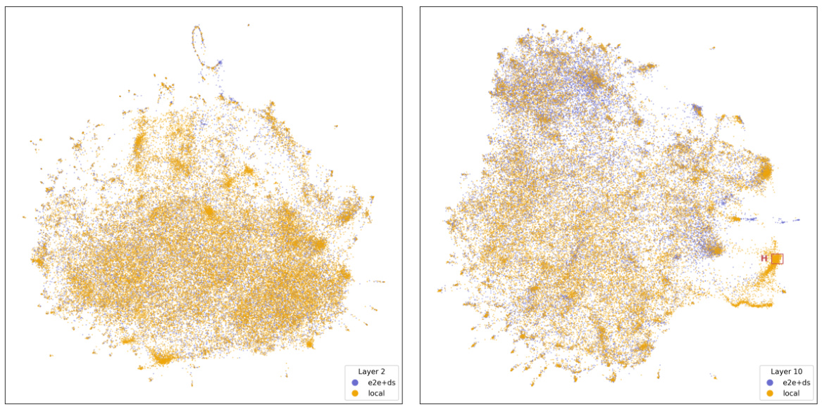
🔼 This figure shows the UMAP plots of Sparse Autoencoders (SAEs) features for layers 2 and 10 of the GPT2-small model. The plots visualize the differences between the features learned by two methods: locally trained SAEs (SAElocal) and end-to-end trained SAEs (SAEe2e+ds). The plots are used to qualitatively analyze and compare the feature distributions obtained from both training approaches. The end-to-end SAEs aim to identify features that are functionally important for explaining network behavior. By comparing the UMAP visualizations, we gain insights into how the methods differ in learning features, in terms of feature distribution and clustering.
read the caption
Figure 20: UMAP plot of SAEe2e+ds and SAElocal features for layers 2 and 10 on runs with similar CE loss increase in GPT2-small.

🔼 This figure displays a UMAP plot visualizing the features from SAEe2e+ds and SAElocal models. Each point represents a feature, and the color of the point indicates its cosine similarity to the 0th principal component analysis (PCA) direction of the original model’s activations. The plot helps to understand the geometric relationships and differences between features learned by the two types of models in terms of their proximity to the 0th PCA direction.
read the caption
Figure 21: The UMAP plot for SAEe2e+ds and SAElocal directions, with points colored by their cosine similarity to the 0th PCA direction.
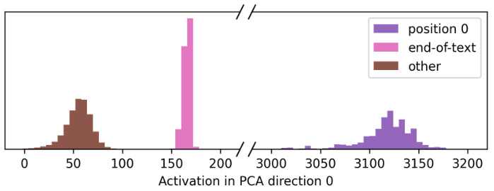
🔼 This figure shows a histogram of the 0th principal component analysis (PCA) component of the activations before layer 10 in the GPT-2 small language model. The histogram is trimodal, with distinct peaks representing three different types of activations: those at position 0, those at end-of-text positions, and others. This indicates that the 0th PCA direction captures a significant portion of the variance in the activation patterns, and that this variance is associated with distinct aspects of the data.
read the caption
Figure 22: A histogram of the 0th PCA component of the activations before layer 10.

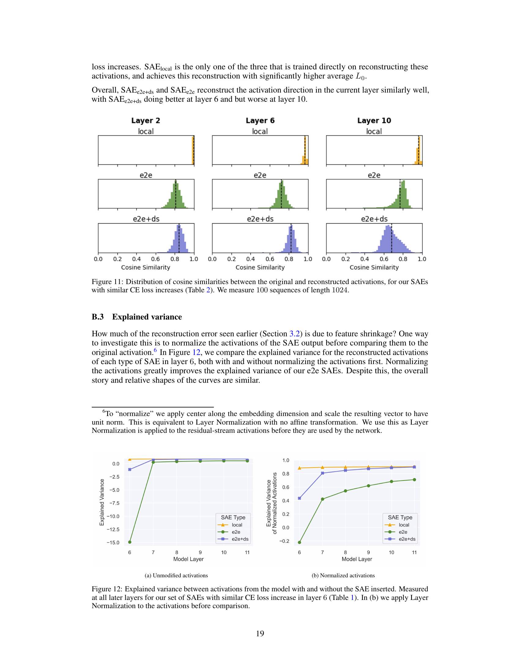
🔼 This figure displays the distribution of cosine similarity scores between original and reconstructed activations for three types of Sparse Autoencoders (SAEs): local, e2e, and e2e+ds. The SAEs were selected based on having similar cross-entropy (CE) loss increases, as detailed in Table 2 of the paper. The analysis was performed on 100 sequences of length 1024. The distributions illustrate how well each SAE type reconstructs the activation directions. A higher concentration of scores closer to 1.0 indicates better reconstruction accuracy.
read the caption
Figure 11: Distribution of cosine similarities between the original and reconstructed activations, for our SAEs with similar CE loss increases (Table 2). We measure 100 sequences of length 1024.

🔼 This figure shows two plots. The left plot shows the correlation between the original and reconstructed activations for each of the top 25 principal components (PCs) before layer 10 in the GPT2-small model. The right plot shows the KL divergence between the original model’s output distribution and the model’s output distribution after selectively removing (ablating) the activation in each of the top 25 PCs. These results demonstrate how well the different types of sparse autoencoders (SAEs) preserve information in these PC directions, and also how functionally important these directions are to the overall network function.
read the caption
Figure 23: For each PCA direction before layer 10 we measure two qualities. The first is how faithfully SAElocal and SAEe2e+ds reconstruct that direction by measuring correlation coefficient. The second is how functionally-important the direction is, as measured by how much the output of the model changes when resample ablating the direction.

🔼 This figure compares three different methods for training sparse autoencoders (SAEs): SAElocal, SAEe2e, and SAEe2e+ds. The top panel illustrates the loss functions used in each method. SAElocal minimizes the mean squared error (MSE) between the input and output activations. SAEe2e minimizes the Kullback-Leibler (KL) divergence between the output distributions of the original model and the model with SAE activations. SAEe2e+ds combines both KL divergence and MSE reconstruction loss. The bottom panel shows Pareto curves that illustrate the trade-off between the number of features used and the cross-entropy (CE) loss increase for each method. E2e-SAEs outperform standard SAEs by requiring fewer features and achieving better CE loss increase.
read the caption
Figure 1: Top: Diagram comparing the loss terms used to train each type of SAE. Each arrow is a loss term which compares the activations represented by circles. SAElocal uses MSE reconstruction loss between the SAE input and the SAE output. SAEe2e uses KL-divergence on the logits. SAEe2e+ds (end-to-end + downstream reconstruction) uses KL-divergence in addition to the sum of the MSE reconstruction losses at all future layers. All three are additionally trained with a L₁ sparsity penalty (not pictured). Bottom: Pareto curves for three different types of GPT2-small layer 6 SAEs as the sparsity coefficient is varied. E2e-SAEs require fewer features per datapoint (i.e. have a lower Lo) and fewer features over the entire dataset (i.e. have a low number of alive dictionary elements). GPT2-small has a CE loss of 3.139 over our evaluation set.
More on tables

🔼 This table presents a comparison of three different types of Sparse Autoencoders (SAEs) trained on layer 6 of a GPT-2 small language model. The SAEs are trained with different loss functions to emphasize different aspects of feature learning: local reconstruction loss, end-to-end KL divergence loss, and end-to-end KL divergence with downstream reconstruction loss. The table compares the sparsity coefficient (λ), the average number of active features per data point (Lo), the total number of active dictionary elements, and the increase in cross-entropy loss (CE Loss Increase) for each SAE type. The values show that end-to-end SAEs require fewer features to achieve similar levels of performance, suggesting that they are more efficient at capturing functionally important features.
read the caption
Table 1: Three SAEs from layer 6 with similar CE loss increases are analyzed in detail.
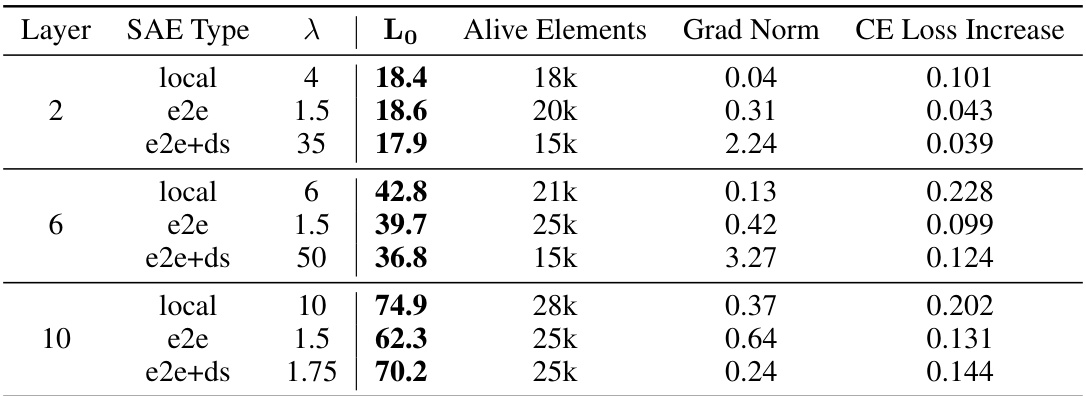
🔼 This table compares three different types of Sparse Autoencoders (SAEs) trained on layer 6 of a GPT2-small model. The SAEs are trained with different loss functions to minimize either Mean Squared Error (MSE) or Kullback-Leibler (KL) divergence, along with a sparsity penalty (L1). The table shows the sparsity coefficient (λ), the average number of active SAE features per datapoint (Lo), the total number of ‘alive’ dictionary elements, and the resulting cross-entropy (CE) loss increase compared to the original model. The aim is to highlight the trade-offs and relative performance of each SAE type.
read the caption
Table 1: Three SAEs from layer 6 with similar CE loss increases are analyzed in detail.
🔼 This table presents a comparison of three different types of Sparse Autoencoders (SAEs) trained on layer 6 of a GPT2-small model. The SAEs are categorized as Local, End-to-end, and End-to-end + downstream. For each SAE type, the table lists the sparsity coefficient (λ), the average number of features activated per data point (Lo), the total number of active dictionary elements, and the increase in cross-entropy loss. The purpose of the table is to illustrate the Pareto improvement of the end-to-end methods over the baseline local SAE method.
read the caption
Table 1: Three SAEs from layer 6 with similar CE loss increases are analyzed in detail.

🔼 This table presents the L2 ratio for three types of Sparse Autoencoders (SAEs): local, e2e, and e2e+ds. The L2 ratio is a measure of feature suppression, calculated as the ratio of the L2 norm of the SAE’s output to the L2 norm of the input. The table shows the L2 ratio for position 0 (the most suppressed position) and positions greater than 0. It compares results at layers 2, 6, and 10. Lower ratios indicate higher suppression.
read the caption
Table 5: L2 Ratio for the SAEs of similar CE loss increase, as in Table 2.

🔼 This table shows the training time taken for three different types of Sparse Autoencoders (SAEs) on three different layers of the GPT2-small language model. The training times are shown in hours and minutes, and are broken down by the type of SAE used: SAElocal, SAEe2e, and SAEe2e+ds. The training time for e2e SAEs was approximately 2-3.5 times longer than the SAElocal training times, and the differences in training time between SAEe2e and SAEe2e+ds were negligible.
read the caption
Table 6: Training times for different layers and SAE training methods using a single NVIDIA A100 GPU on the residual stream of GPT2-small at layer 6. All SAEs are trained on 400k samples of context length 1024, with a dictionary size of 60x the residual stream size of 768.

🔼 This table shows the faithfulness scores for different SAE types (local, e2e, e2e+ds) across various subject-verb agreement tasks (simple, across participle phrase, across relative clause, within relative clause) at different layers (2, 6, 10). Faithfulness measures how well the model performs compared to a random baseline when the original activations are replaced with SAE outputs. A score of 100% means that the SAE perfectly preserves the model’s performance. The table presents the results for runs with similar CE loss increase and similar Lo, demonstrating how different SAE training methods impact the preservation of functionally relevant information in the model’s activations for downstream tasks.
read the caption
Table 7: Faithfulness on subject-verb agreement when replacing the activations with SAE outputs.
Full paper#
