TL;DR#
Current AI models like CLIP, while effective, produce high-dimensional, difficult-to-interpret outputs, hindering understanding of their decision-making processes. This lack of transparency is a major obstacle for applications needing trustworthiness and accountability. The resulting opacity also makes it difficult to identify and correct biases or errors in the model.
SpLiCE overcomes this challenge using a novel method to decompose CLIP’s dense representations into sparse linear combinations of human-interpretable concepts. This task-agnostic approach maintains high performance on downstream tasks while significantly improving interpretability. The authors demonstrate the method’s effectiveness in detecting spurious correlations and editing AI models, opening new possibilities for trustworthy AI development and use.
Key Takeaways#
Why does it matter?#
This paper is crucial for researchers seeking to enhance the interpretability of complex AI models. SpLiCE offers a novel, task-agnostic approach for improving understanding of AI’s decision-making processes. This work directly addresses the growing demand for transparency in AI systems, paving the way for more trustworthy and reliable AI applications. The method’s ability to detect spurious correlations and allow model editing will greatly benefit a variety of research fields, prompting further exploration of interpretable AI.
Visual Insights#

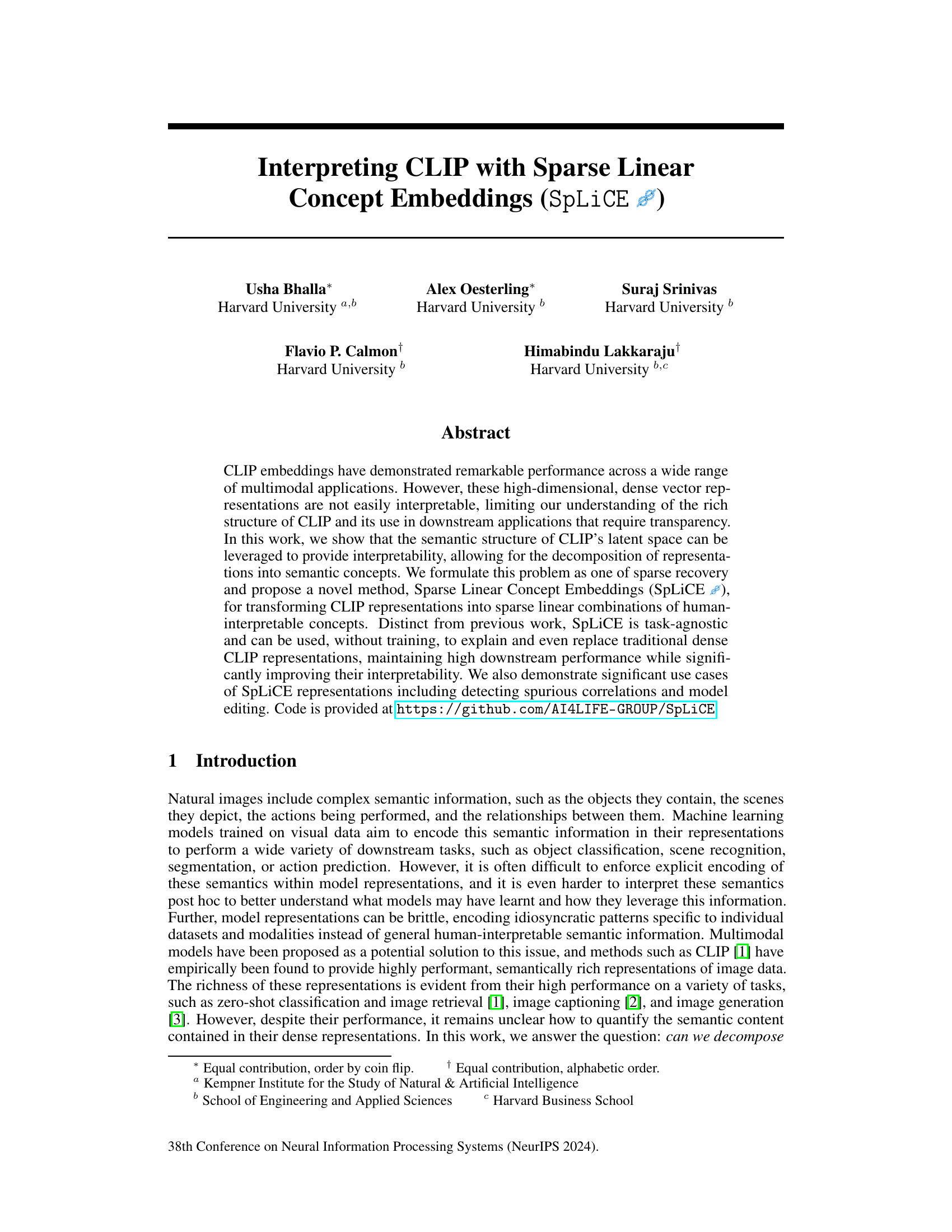
🔼 The figure illustrates the SpLiCE method. Dense CLIP image representations are transformed into sparse, interpretable concept decompositions. SpLiCE uses a sparse, nonnegative linear solver to find the optimal sparse combination of concepts (from a large, overcomplete concept set) that best represents the original CLIP embedding. The input is a set of dense image representations from CLIP. The output is a set of sparse semantic decompositions, where each decomposition consists of a small number of weighted concepts. The process leverages an overcomplete concept set to enable flexible and sparse representations.
read the caption
Figure 1: Visualization of SpLiCE, which converts dense, uninterpretable CLIP representations (z) into sparse semantic decompositions (w) by solving for a sparse nonnegative linear combination over an overcomplete concept set (C).

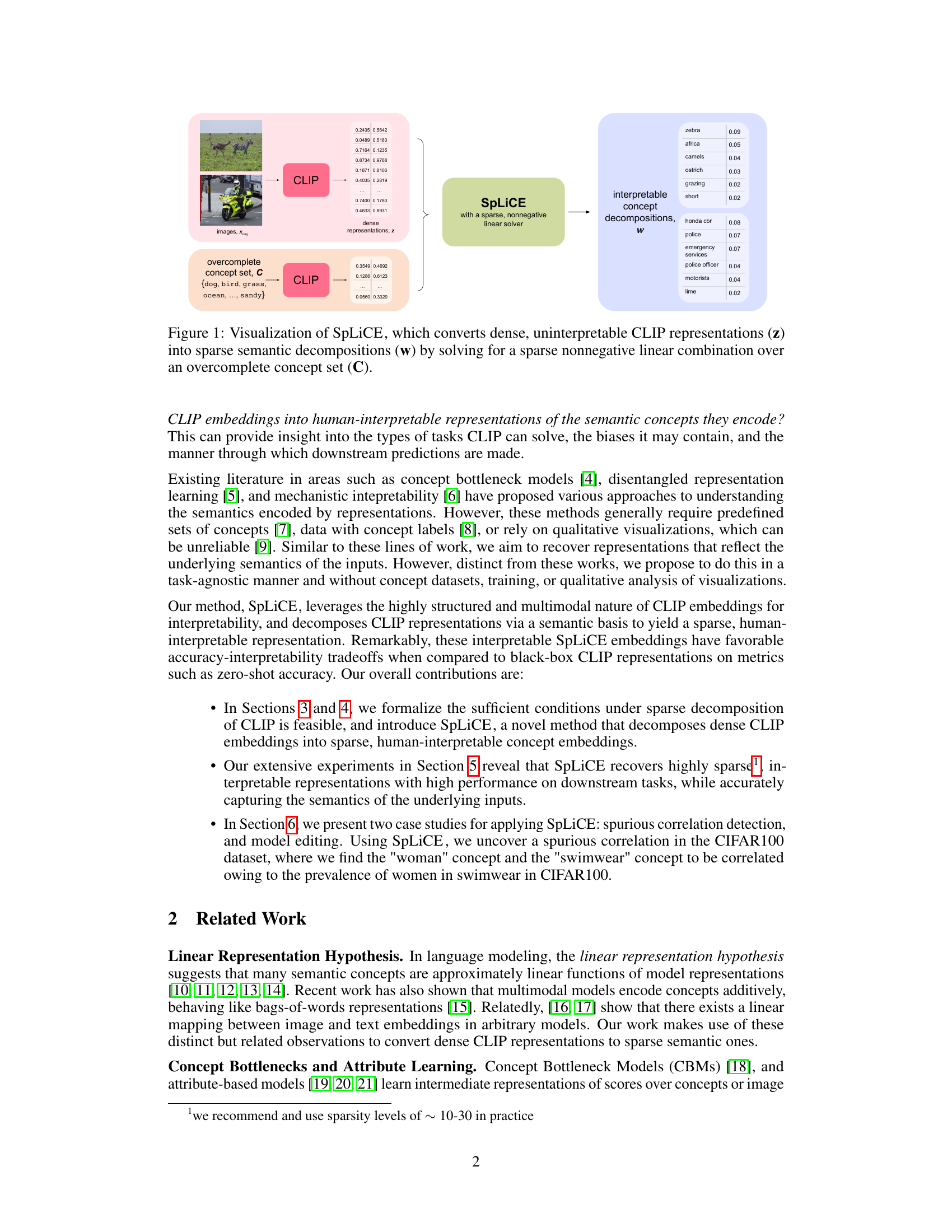
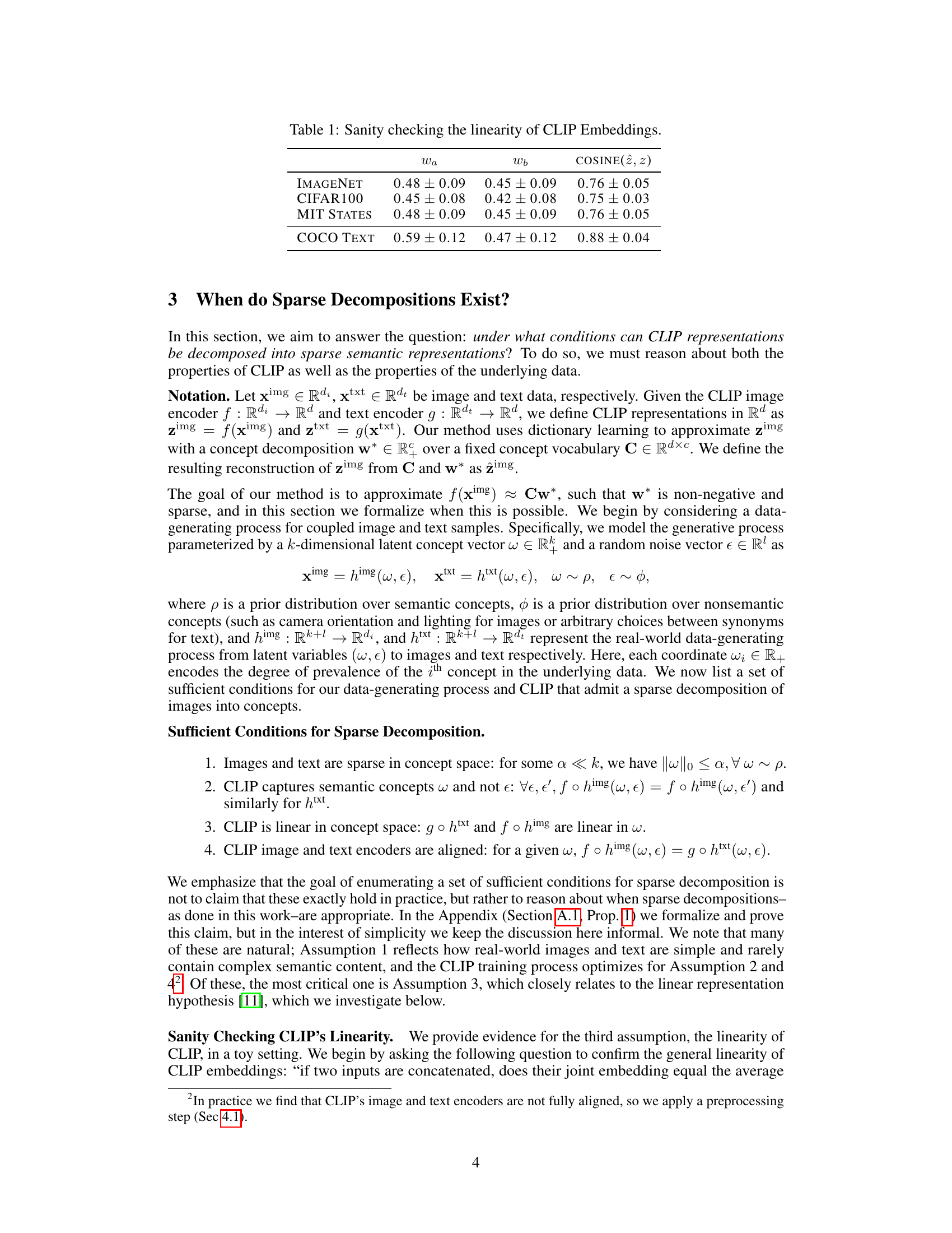
🔼 This table presents the results of a sanity check to evaluate the linearity assumption of CLIP embeddings. The experiment combines two images or text inputs and compares their joint CLIP embedding to the average of their individual embeddings. The table shows the weights (wₐ and wբ) obtained by solving the linear equation and the cosine similarity between the combined embedding and the weighted average of individual embeddings for four different datasets (ImageNet, CIFAR100, MIT States, COCO Text). The results show that the weights are close to 0.5 and the cosine similarity is high across all datasets, providing evidence that CLIP embeddings exhibit approximately linear behavior in concept space.
read the caption
Table 1: Sanity checking the linearity of CLIP Embeddings.
In-depth insights#
SpLiCE: Core Idea#
SpLiCE’s core idea centers on enhancing the interpretability of CLIP’s dense image embeddings by decomposing them into sparse linear combinations of human-understandable concepts. Instead of relying on complex, task-specific methods, SpLiCE leverages the inherent semantic structure within CLIP’s latent space. This is achieved through a novel sparse recovery formulation, enabling a task-agnostic approach. The method’s strength lies in its ability to transform dense CLIP representations into sparse, interpretable concept decompositions without requiring any training or predefined concept datasets. This makes SpLiCE uniquely powerful for understanding CLIP’s internal workings, identifying biases, and even editing its behavior. By representing images as sparse combinations of concepts, SpLiCE significantly improves interpretability while maintaining high downstream performance in various tasks. The use of an overcomplete concept dictionary allows SpLiCE to capture a wide range of semantic information and avoid the limitations of smaller, task-specific concept sets. The resulting sparse representations offer valuable insights into both the functioning of the model and the underlying data. This is achieved by framing the problem as sparse recovery, using an overcomplete dictionary of 1 and 2 word concepts derived from text captions.
SpLiCE: Method#
The SpLiCE method section would detail the algorithm’s inner workings, explaining how it transforms dense CLIP representations into sparse, interpretable concept embeddings. It would likely start by formalizing the problem as sparse recovery and then describe the specific optimization strategy used (e.g., a non-negative LASSO solver). Key design choices such as the construction of the concept vocabulary (e.g., using 1- and 2-word phrases from a large corpus), addressing potential modality gaps between image and text representations, and the specific optimization algorithm parameters (e.g., sparsity levels and regularization strength) would be carefully explained. The method would also address how the algorithm handles the overcomplete nature of the concept set, ensuring the solution is both sparse and interpretable. A crucial component would be a discussion of the algorithm’s efficiency and scalability, noting the computational cost and feasibility for processing large datasets. The choice of the solver and how it’s adapted for the specific requirements of SpLiCE would be highlighted. Finally, the section would likely conclude by outlining the process of generating and interpreting SpLiCE outputs, perhaps using visualization techniques to illustrate the resulting sparse concept decompositions. The mathematical notations and details about the optimization problem would likely be included for reproducibility.
Evaluation Metrics#
A robust evaluation of any model demands a multifaceted approach, and the choice of metrics significantly influences the interpretation of results. For a model focused on interpretability, like the one described, accuracy alone is insufficient. We need metrics that assess the quality of the generated explanations. Sparsity of the concept embeddings is crucial, as it directly relates to human interpretability. However, excessive sparsity could compromise accuracy. Thus, a balance between sparsity and accuracy must be carefully considered, possibly using metrics such as the L1 norm of the concept vectors and zero-shot classification accuracy. Furthermore, semantic relevance should be quantitatively evaluated; how well do the extracted concepts reflect the actual semantic content of the input? This might involve comparing against human-generated labels or using techniques like cosine similarity between concept embeddings and word embeddings. Ultimately, the most informative evaluation incorporates both quantitative metrics and qualitative analysis of generated explanations to provide a comprehensive understanding of the model’s performance.
Ablation Studies#
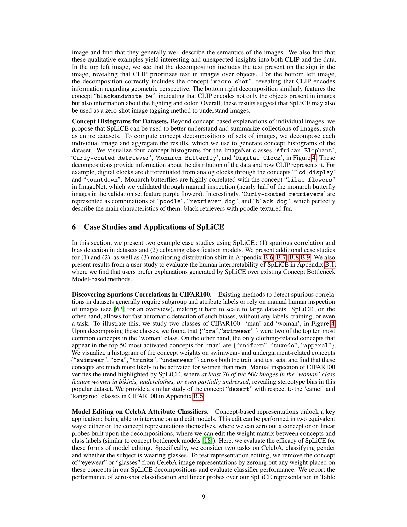
An ablation study systematically removes components of a model or system to assess their individual contributions. In the context of a research paper, an ablation study on a method for interpreting CLIP embeddings would likely investigate the impact of various design choices. For example, the study could analyze the effectiveness of the chosen concept vocabulary. Removing the semantic concept vocabulary and substituting random or learned vocabularies would gauge the impact of human interpretability versus randomly selected concepts or those learned through an unsupervised method. The study might also examine the role of sparsity in the decompositions, comparing the performance of sparse versus dense solutions and investigating the influence of non-negativity constraints on interpretability and accuracy. The importance of modality alignment between images and texts could be explored by testing the algorithm without the alignment step, to identify its contribution to overall accuracy. This rigorous approach allows researchers to pinpoint which aspects of their method are essential for achieving strong results and which are peripheral, offering a robust analysis of the model’s critical components.
Future Work#
The paper’s lack of a dedicated ‘Future Work’ section presents an opportunity for expansion. Extending SpLiCE to handle more complex semantic structures beyond single or double-word concepts is crucial. This might involve exploring hierarchical representations or incorporating richer linguistic features. Investigating the impact of different concept dictionaries on SpLiCE’s performance, particularly those tailored to specific domains or tasks, is also important. A thorough analysis of SpLiCE’s robustness to noise and variations in data should be performed. Benchmarking against other interpretability methods on a wider range of datasets and tasks would strengthen the findings. Finally, exploring applications where SpLiCE’s sparse representations can improve efficiency or reduce computational cost warrants further investigation. These advancements would further solidify SpLiCE’s position as a leading interpretability tool for multimodal models.
More visual insights#
More on figures

🔼 This figure shows six example images from the MSCOCO dataset, each with its corresponding caption and top seven concepts identified using SpLiCE. The concept decompositions illustrate how SpLiCE represents the image semantics in terms of a sparse combination of human-interpretable concepts. Note that each image actually has a decomposition with 7 to 20 concepts; only the top seven are displayed for visual clarity.
read the caption
Figure 2: Example images from MSCOCO shown with their captions below and their concept decompositions on the right. We display the top seven concepts for visualization purposes, but images in the figure had decompositions with 7–20 concepts.
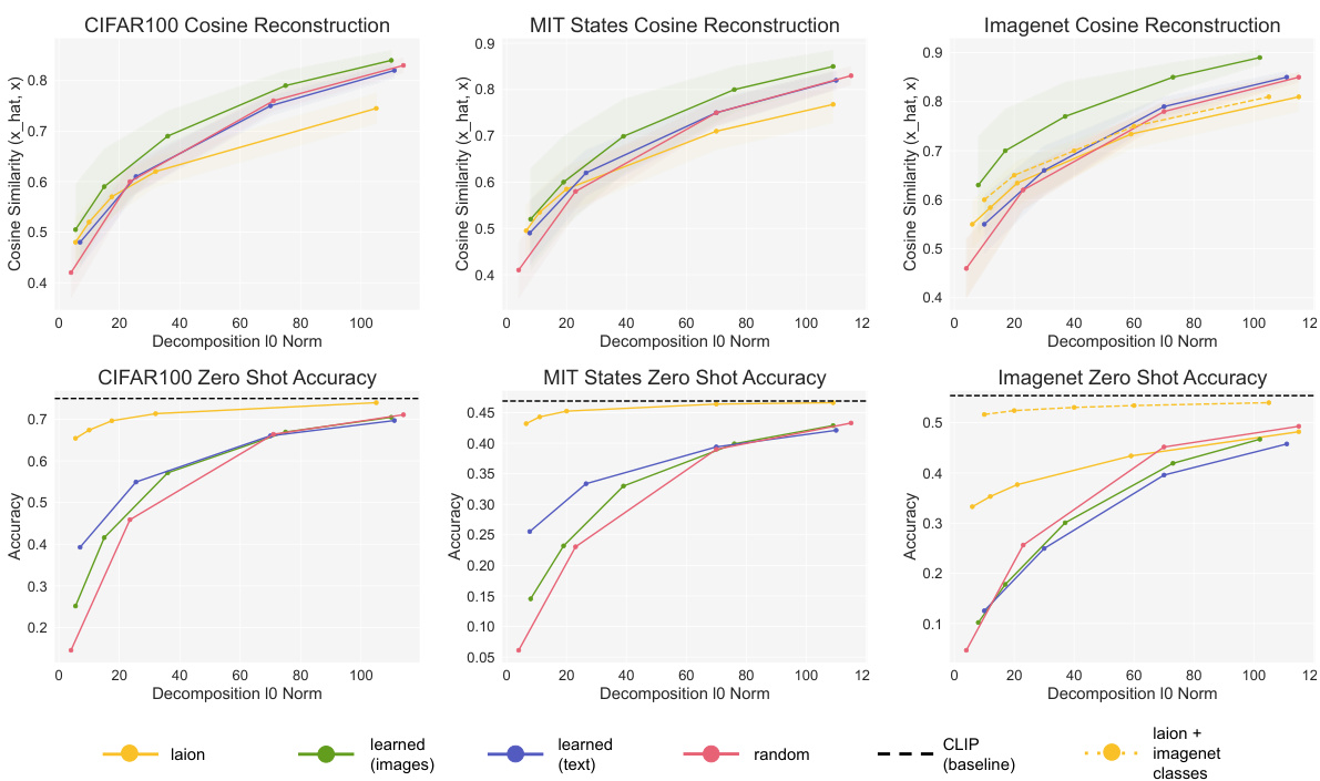
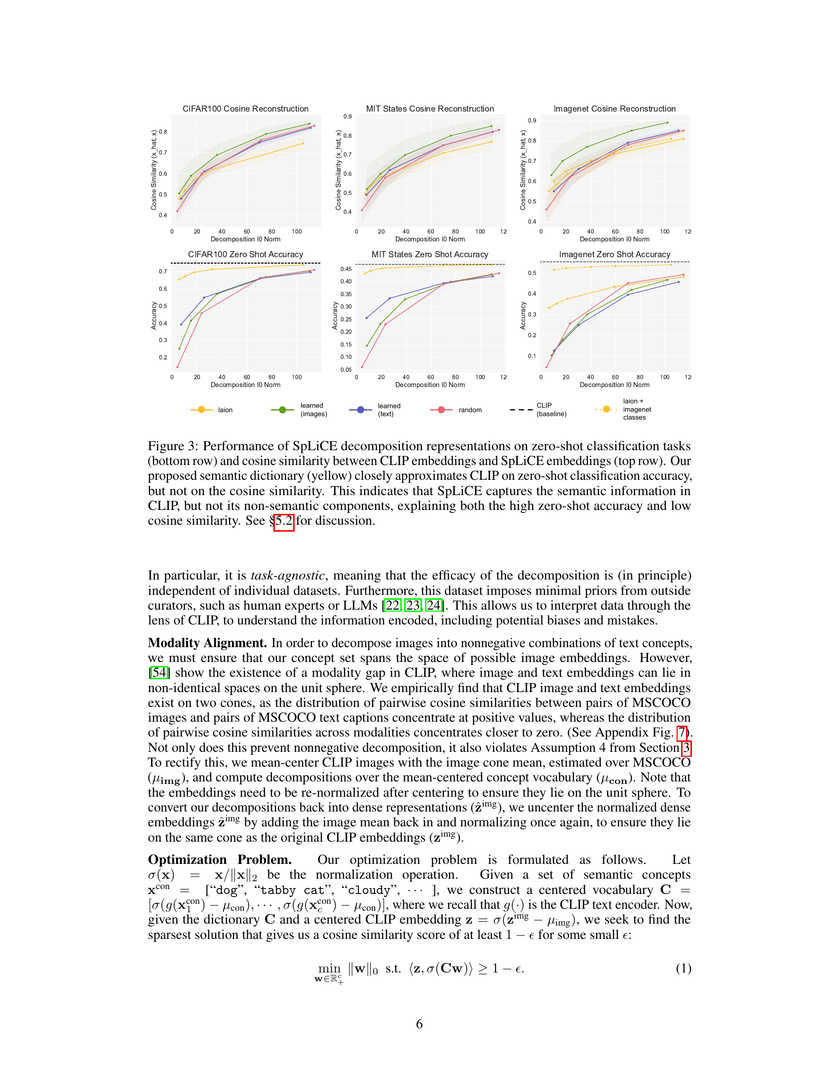
🔼 This figure displays the performance of SpLiCE on zero-shot classification and cosine similarity reconstruction tasks. The top row shows the cosine similarity between the original CLIP embeddings and the SpLiCE representations for different datasets (CIFAR100, MIT States, and ImageNet). The bottom row shows the zero-shot classification accuracy on the same datasets. The results indicate that SpLiCE, using a semantic dictionary (yellow line), achieves high zero-shot accuracy, comparable to CLIP (black line), while demonstrating lower cosine similarity. This suggests that SpLiCE effectively captures the semantic information in CLIP while filtering out non-semantic components.
read the caption
Figure 3: Performance of SpLiCE decomposition representations on zero-shot classification tasks (bottom row) and cosine similarity between CLIP embeddings and SpLiCE embeddings (top row). Our proposed semantic dictionary (yellow) closely approximates CLIP on zero-shot classification accuracy, but not on the cosine similarity. This indicates that SpLiCE captures the semantic information in CLIP, but not its non-semantic components, explaining both the high zero-shot accuracy and low cosine similarity. See §5.2 for discussion.

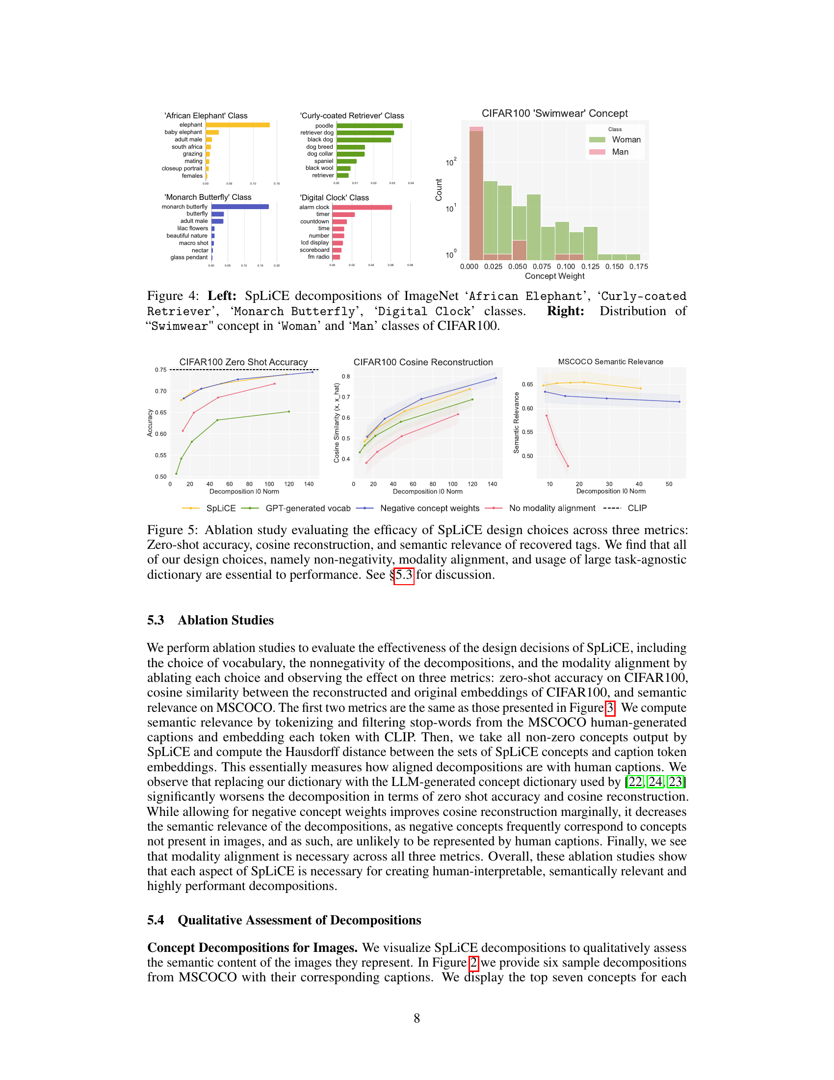
🔼 The figure shows the top concepts identified by SpLiCE for four different ImageNet classes, demonstrating the method’s ability to capture semantically meaningful components in the data. It also visualizes the distribution of the ‘Swimwear’ concept within the ‘Woman’ and ‘Man’ classes of the CIFAR-100 dataset, highlighting the presence of potential biases in the dataset.
read the caption
Figure 4: Left: SpLiCE decompositions of ImageNet ‘African Elephant’, ‘Curly-coated Retriever’, ‘Monarch Butterfly’, ‘Digital Clock’ classes. Right: Distribution of “Swimwear” concept in ‘Woman’ and ‘Man’ classes of CIFAR100.

🔼 This figure shows the performance of SpLiCE decompositions in zero-shot classification tasks and cosine similarity with CLIP embeddings. The top row displays the cosine similarity between original CLIP embeddings and SpLiCE representations across different datasets (CIFAR100, MIT States, and ImageNet). The bottom row shows the zero-shot accuracy of SpLiCE representations on the same datasets. The results indicate SpLiCE successfully captures semantic information while discarding non-semantic components, leading to high zero-shot accuracy despite lower cosine similarity to the original CLIP embeddings. The yellow line in the graphs represents the performance using SpLiCE’s proposed semantic dictionary.
read the caption
Figure 3: Performance of SpLiCE decomposition representations on zero-shot classification tasks (bottom row) and cosine similarity between CLIP embeddings and SpLiCE embeddings (top row). Our proposed semantic dictionary (yellow) closely approximates CLIP on zero-shot classification accuracy, but not on the cosine similarity. This indicates that SpLiCE captures the semantic information in CLIP, but not its non-semantic components, explaining both the high zero-shot accuracy and low cosine similarity. See §5.2 for discussion.
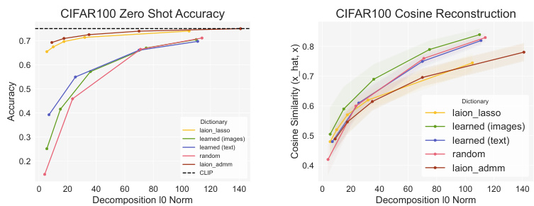
🔼 This figure displays the performance of SpLiCE decompositions on zero-shot classification and cosine similarity reconstruction tasks across multiple datasets. It compares the performance of SpLiCE using a semantic concept vocabulary to baselines using random and learned vocabularies. The results show that SpLiCE’s semantic dictionary achieves comparable zero-shot classification accuracy to CLIP but lower cosine similarity. This suggests that SpLiCE captures the semantic meaning while discarding non-semantic aspects of the CLIP embeddings.
read the caption
Figure 3: Performance of SpLiCE decomposition representations on zero-shot classification tasks (bottom row) and cosine similarity between CLIP embeddings and SpLiCE embeddings (top row). Our proposed semantic dictionary (yellow) closely approximates CLIP on zero-shot classification accuracy, but not on the cosine similarity. This indicates that SpLiCE captures the semantic information in CLIP, but not its non-semantic components, explaining both the high zero-shot accuracy and low cosine similarity. See §5.2 for discussion.
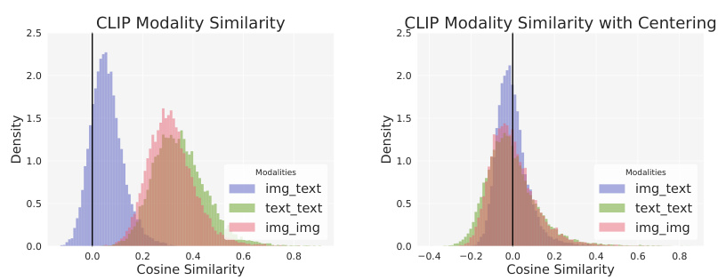
🔼 This figure shows the distribution of cosine similarity scores between different pairs of modalities (image-image, text-text, and image-text) in the MSCOCO dataset. The left panel shows the distribution before any modality alignment, illustrating a clear separation between modalities with higher similarity within each modality than across them. The right panel displays the same distribution after applying a modality alignment technique (mean-centering), showing a centered distribution around zero, indicating successful alignment of the modalities in the vector space.
read the caption
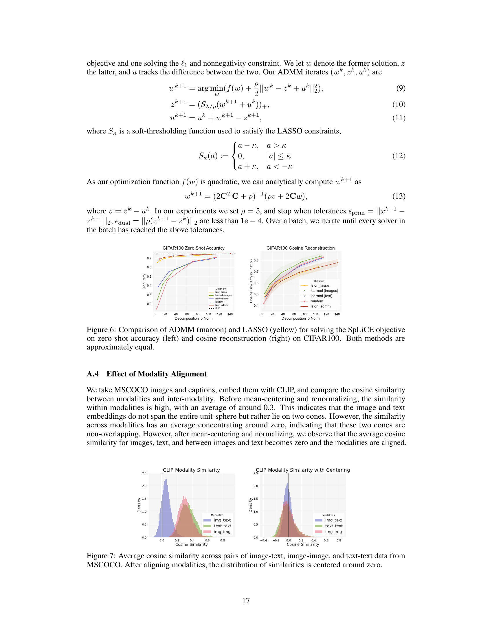
Figure 7: Average cosine similarity across pairs of image-text, image-image, and text-text data from MSCOCO. After aligning modalities, the distribution of similarities is centered around zero.

🔼 This figure shows the results of experiments evaluating the performance of SpLiCE on zero-shot classification and the similarity between SpLiCE and CLIP embeddings. The results indicate that SpLiCE, using its proposed semantic dictionary, achieves high accuracy in zero-shot classification, comparable to CLIP. However, the cosine similarity between SpLiCE and CLIP embeddings is lower, suggesting SpLiCE captures semantic information but not non-semantic components of CLIP.
read the caption
Figure 3: Performance of SpLiCE decomposition representations on zero-shot classification tasks (bottom row) and cosine similarity between CLIP embeddings and SpLiCE embeddings (top row). Our proposed semantic dictionary (yellow) closely approximates CLIP on zero-shot classification accuracy, but not on the cosine similarity. This indicates that SpLiCE captures the semantic information in CLIP, but not its non-semantic components, explaining both the high zero-shot accuracy and low cosine similarity. See §5.2 for discussion.
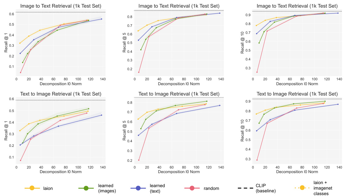
🔼 This figure shows the performance of SpLiCE decompositions on zero-shot classification and the cosine similarity between CLIP and SpLiCE embeddings across different datasets. The top row displays the cosine similarity, showing that SpLiCE’s concept-based representations closely match CLIP’s zero-shot classification performance (bottom row) but not the raw cosine similarity. This demonstrates that SpLiCE successfully captures the semantic aspects of CLIP representations while discarding non-semantic information, leading to high accuracy with improved interpretability.
read the caption
Figure 3: Performance of SpLiCE decomposition representations on zero-shot classification tasks (bottom row) and cosine similarity between CLIP embeddings and SpLiCE embeddings (top row). Our proposed semantic dictionary (yellow) closely approximates CLIP on zero-shot classification accuracy, but not on the cosine similarity. This indicates that SpLiCE captures the semantic information in CLIP, but not its non-semantic components, explaining both the high zero-shot accuracy and low cosine similarity. See §5.2 for discussion.

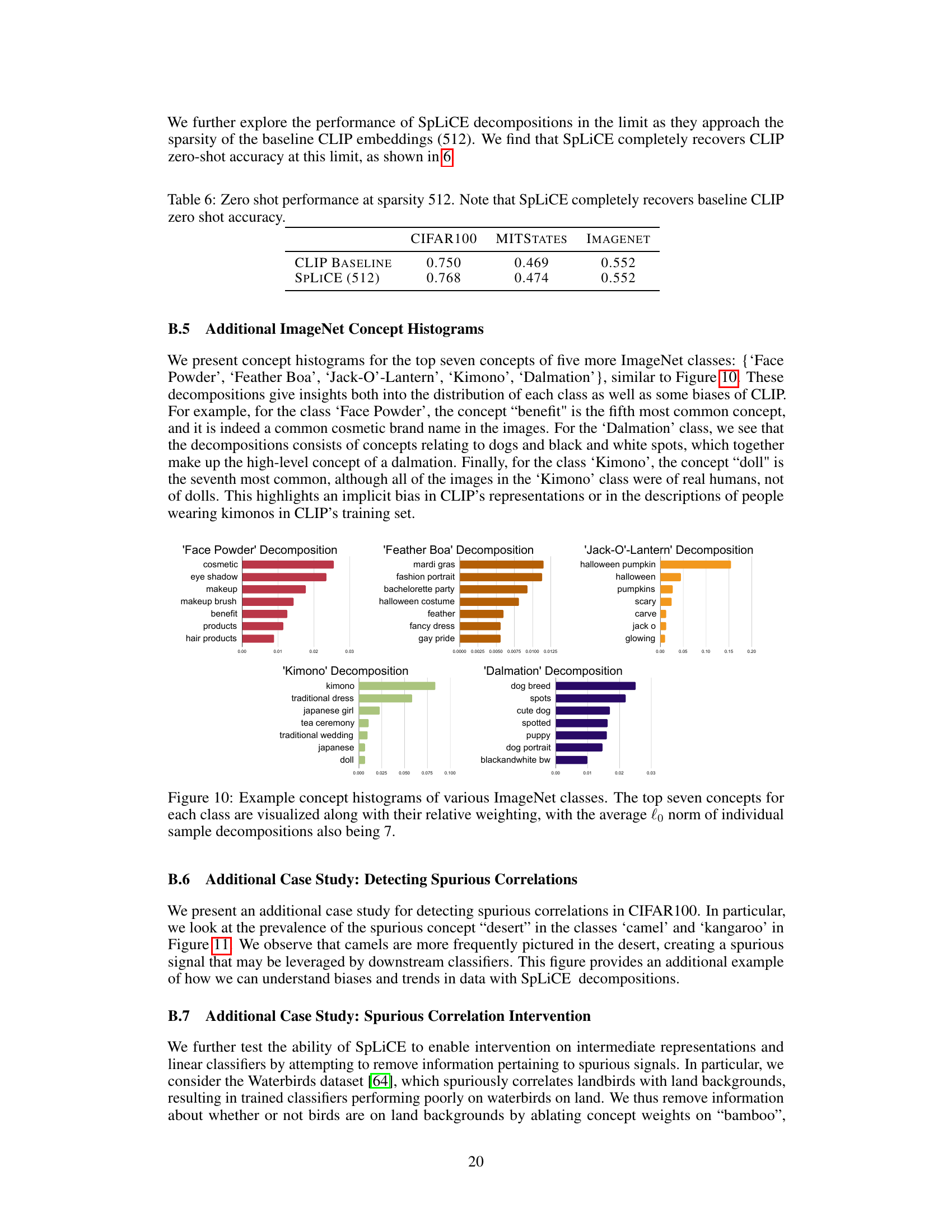
🔼 This figure shows bar charts visualizing the top seven concepts with their weights for five different ImageNet classes: ‘Face Powder’, ‘Feather Boa’, ‘Jack-O’-Lantern’, ‘Kimono’, and ‘Dalmatian’. Each bar chart represents a class, showing the relative importance of each concept in characterizing that class, according to SpLiCE. The figure highlights the interpretability of SpLiCE by showing how the algorithm decomposes each image into a sparse combination of human-understandable concepts. For example, in the ‘Dalmatian’ class, the top concepts are dog breed, spots, and black-and-white, which are highly relevant to the visual characteristics of Dalmatians. The average l0 norm of 7 indicates that, on average, each image is represented by 7 concepts.
read the caption
Figure 10: Example concept histograms of various ImageNet classes. The top seven concepts for each class are visualized along with their relative weighting, with the average l0 norm of individual sample decompositions also being 7.
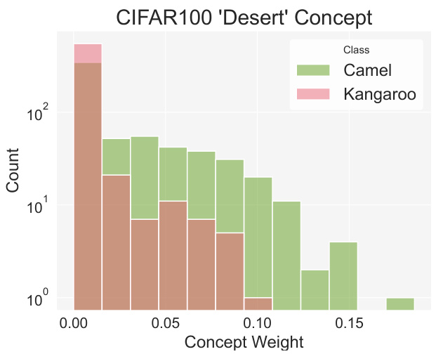
🔼 This histogram displays the distribution of the concept weight for ‘desert’ across the two CIFAR100 classes, ‘Camel’ and ‘Kangaroo’. It illustrates the higher prevalence of the ‘desert’ concept in images of camels compared to kangaroos, suggesting a potential spurious correlation between the presence of camels and desert environments in this dataset.
read the caption
Figure 11: Distribution of “Desert

🔼 This figure visualizes how the prevalence of convertibles and yellow cars in the Stanford Cars dataset changes over the years. The solid lines represent the actual percentage of convertibles and yellow cars in each year, while the dotted lines show the corresponding concept weights obtained using SpLiCE. The close alignment between the actual prevalence and SpLiCE concept weights indicates that SpLiCE accurately captures the temporal trends in these car attributes.
read the caption
Figure 12: Visualization of the presence of convertibles (pink lines) and yellow cars (yellow lines) in Stanford Cars over time. SpLiCE concept weights (dotted) closely track the groundtruth concept prevalence (solid) for both concepts.
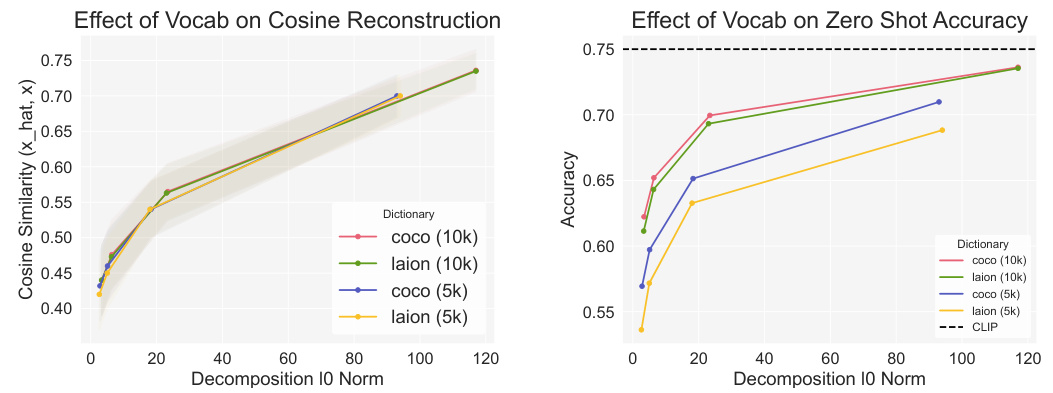
🔼 This figure presents the results of experiments evaluating SpLiCE’s performance on zero-shot image classification and the similarity between its representations and those from original CLIP. The top row shows cosine similarity, demonstrating that SpLiCE (using a learned semantic dictionary) closely matches the original CLIP representations in zero-shot classification but significantly differs in terms of cosine similarity. The bottom row shows the zero-shot accuracy, which remains high even when employing the SpLiCE semantic concept dictionary. This suggests that SpLiCE successfully captures the semantic meaning in CLIP embeddings without replicating its non-semantic aspects.
read the caption
Figure 3: Performance of SpLiCE decomposition representations on zero-shot classification tasks (bottom row) and cosine similarity between CLIP embeddings and SpLiCE embeddings (top row). Our proposed semantic dictionary (yellow) closely approximates CLIP on zero-shot classification accuracy, but not on the cosine similarity. This indicates that SpLiCE captures the semantic information in CLIP, but not its non-semantic components, explaining both the high zero-shot accuracy and low cosine similarity. See §5.2 for discussion.

🔼 The figure illustrates the SpLiCE method. It shows how dense CLIP image embeddings are converted into sparse, interpretable representations. The process involves finding a sparse, non-negative linear combination of a set of human-interpretable concepts to approximate the original CLIP embedding. This is represented visually with the input image, its dense CLIP representation (z), the sparse concept decomposition (w) produced by SpLiCE, and the overcomplete concept set (C) that the linear combination is drawn from.
read the caption
Figure 1: Visualization of SpLiCE, which converts dense, uninterpretable CLIP representations (z) into sparse semantic decompositions (w) by solving for a sparse nonnegative linear combination over an overcomplete concept set (C).

🔼 This figure shows the performance of SpLiCE decompositions on zero-shot classification tasks and the cosine similarity between CLIP and SpLiCE embeddings across three datasets: CIFAR100, MIT States, and ImageNet. The top row displays cosine similarity between original CLIP embeddings and SpLiCE representations with varying sparsity levels. The bottom row presents the zero-shot classification accuracy for the same representations. The results indicate that SpLiCE effectively captures the semantic information from CLIP, achieving high zero-shot accuracy while maintaining a relatively low cosine similarity to the original embeddings. This suggests SpLiCE is successfully disentangling semantic information from non-semantic aspects of CLIP’s dense representations.
read the caption
Figure 3: Performance of SpLiCE decomposition representations on zero-shot classification tasks (bottom row) and cosine similarity between CLIP embeddings and SpLiCE embeddings (top row). Our proposed semantic dictionary (yellow) closely approximates CLIP on zero-shot classification accuracy, but not on the cosine similarity. This indicates that SpLiCE captures the semantic information in CLIP, but not its non-semantic components, explaining both the high zero-shot accuracy and low cosine similarity. See §5.2 for discussion.
More on tables
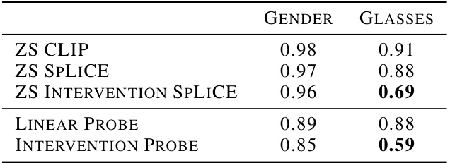
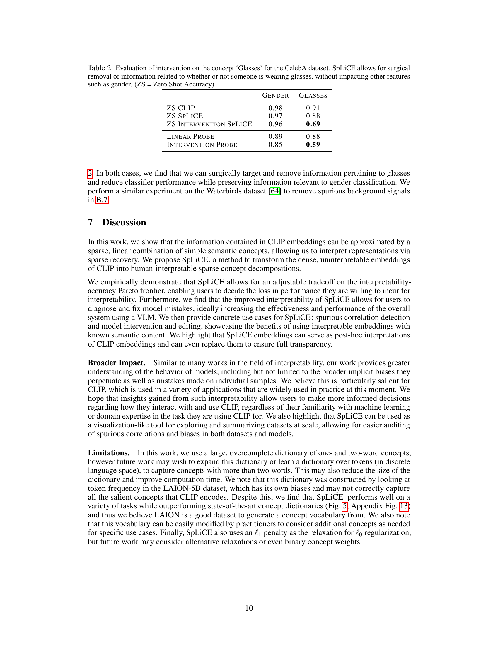
🔼 This table presents the results of an experiment on the CelebA dataset to evaluate the impact of removing the ‘Glasses’ concept using SpLiCE. It compares the zero-shot accuracy (ZS) of CLIP, SpLiCE, and SpLiCE with intervention on two tasks: Gender and Glasses classification. The intervention involves removing the ‘Glasses’ concept, demonstrating that SpLiCE can surgically remove specific information without affecting other features. Linear probes were also used to assess the impact of removing the ‘Glasses’ concept on model performance.
read the caption
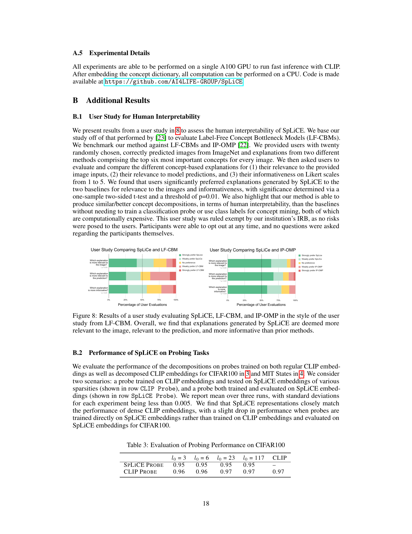
Table 2: Evaluation of intervention on the concept 'Glasses' for the CelebA dataset. SpLiCE allows for surgical removal of information related to whether or not someone is wearing glasses, without impacting other features such as gender. (ZS = Zero Shot Accuracy)

🔼 This table presents the results of probing experiments conducted on the CIFAR100 dataset. Two types of probes were used: one trained on CLIP embeddings and tested on SpLiCE embeddings (CLIP Probe), and one trained and evaluated on SpLiCE embeddings (SpLiCE Probe). The table shows the performance of these probes for various sparsity levels (l0 norms) of the SpLiCE embeddings, ranging from 3 to 117. The performance is measured in terms of accuracy and serves to illustrate the trade-off between interpretability (sparsity) and performance.
read the caption
Table 3: Evaluation of Probing Performance on CIFAR100

🔼 This table presents the results of probing experiments conducted on the MIT States dataset. It compares the performance of probes trained on SpLiCE embeddings and CLIP embeddings. Different levels of sparsity (l0) are tested for SpLiCE, and the performance is measured in terms of accuracy. The results show that SpLiCE embeddings, at different sparsity levels, achieve comparable performance to CLIP embeddings on this probing task.
read the caption
Table 4: Evaluation of Probing Performance on MIT States

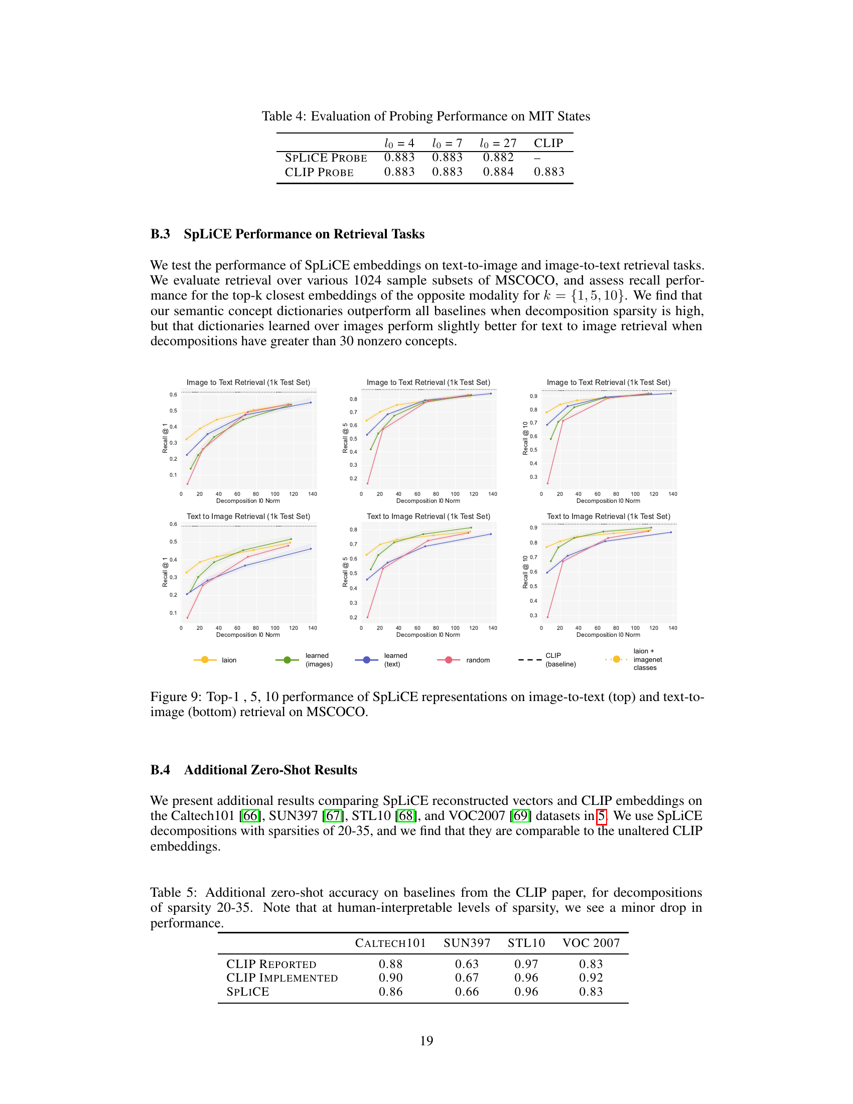
🔼 This table presents additional zero-shot accuracy results obtained using SpLiCE and compares them to the baseline results reported in the original CLIP paper. The results are shown for four datasets: Caltech101, SUN397, STL10, and VOC2007. SpLiCE uses decompositions with sparsity levels between 20 and 35. The table shows that while SpLiCE achieves comparable accuracy to CLIP’s baseline, there is a slight drop in performance when using human-interpretable sparsity levels.
read the caption
Table 5: Additional zero-shot accuracy on baselines from the CLIP paper, for decompositions of sparsity 20-35. Note that at human-interpretable levels of sparsity, we see a minor drop in performance.

🔼 This table presents the zero-shot accuracy results for three different datasets (CIFAR100, MIT States, and ImageNet) when using SpLiCE with a sparsity level of 512. The results show that SpLiCE achieves almost identical performance to the baseline CLIP model at this high sparsity level, demonstrating that SpLiCE can fully recover the performance of CLIP while maintaining its improved interpretability.
read the caption
Table 6: Zero shot performance at sparsity 512. Note that SpLiCE completely recovers baseline CLIP zero shot accuracy.

🔼 This table presents the results of an experiment on the Waterbirds dataset, which aims to mitigate spurious correlations between bird types and their backgrounds (land vs. water). A linear probe model was used for classification. The first row shows the accuracy of the linear probe on landbirds and waterbirds when the model is trained on the original dataset. The second row shows the results after removing information about land backgrounds from the SpLiCE representation of the images, illustrating how this intervention can improve the performance, specifically on waterbirds on land, by reducing bias.
read the caption
Table 7: Evaluation of intervention on spurious correlations for Waterbirds dataset. Removing information about land backgrounds improves worst-case subgroup performance.

🔼 This table shows the cosine similarity between the class distributions for the train, validation, and test splits of the Waterbirds dataset. The values indicate the differences between the distributions. The results show that the validation and test sets are much more similar to each other than either is to the training set, suggesting a potential issue with the distribution of data across splits.
read the caption
Table 8: Study of the differences in distributions between train, validation, and test splits of Waterbirds. The validation and test splits are much more similar to each other than they are to the train split.

🔼 This table presents the weighted average of the concept ‘bamboo’ across different classes (landbird and waterbird) and data splits (train, validation, and test) of the Waterbirds dataset. The values show that the training set has a much higher weighted average for the concept ‘bamboo’ in the landbird class than in the waterbird class. In contrast, the validation and test sets show a more balanced distribution of this concept across both classes. This suggests a potential bias in the training data, where the concept ‘bamboo’ is more strongly associated with landbirds. The table highlights the importance of examining data splits for potential biases that might affect model performance.
read the caption
Table 9: Study of the prevalence of the concept “bamboo” in the different classes and splits of Waterbirds.

🔼 This table presents the results of an experiment evaluating the similarity between antonyms and concepts preceded by ’not’ in CLIP embeddings. Two sets of cosine similarity scores are reported: one without concept centering and one with concept centering. The results indicate that even with centering, CLIP does not place antonyms in opposite directions in its embedding space, as evidenced by high similarity scores between antonyms and between concepts and their negated versions. This suggests that CLIP’s internal representation of semantics may not rely on simple antonym relationships.
read the caption
Table 10: Evaluation of the similarity of antonyms and negative concepts in CLIP.
Full paper#
