TL;DR#
Many scientific applications rely on Bayesian inference with latent variable models. However, obtaining sufficient clean data to effectively train prior distributions, such as diffusion models, can be extremely difficult. Existing methods for training diffusion models typically require large amounts of high-quality data, limiting their applicability in many real-world situations where data is scarce or noisy.
This paper introduces a novel Expectation-Maximization (EM) algorithm to effectively train diffusion models from incomplete and noisy observations. Unlike previous methods, this approach generates proper diffusion models crucial for downstream applications. Additionally, the paper proposes an improved posterior sampling method, enhancing the accuracy of inference results. Through experiments using various datasets, the research demonstrates the effectiveness of the proposed method, showcasing its ability to generate high-quality results even with limited and noisy data. The core contribution is a practical and efficient method to train diffusion models in data-scarce environments.
Key Takeaways#
Why does it matter?#
This paper is important because it presents a novel method for training diffusion models using limited, noisy data, a common challenge in many scientific applications. The improved posterior sampling technique is also a valuable contribution, impacting the wider field of Bayesian inference. This opens avenues for applying diffusion models to new problems where large clean datasets are unavailable.
Visual Insights#
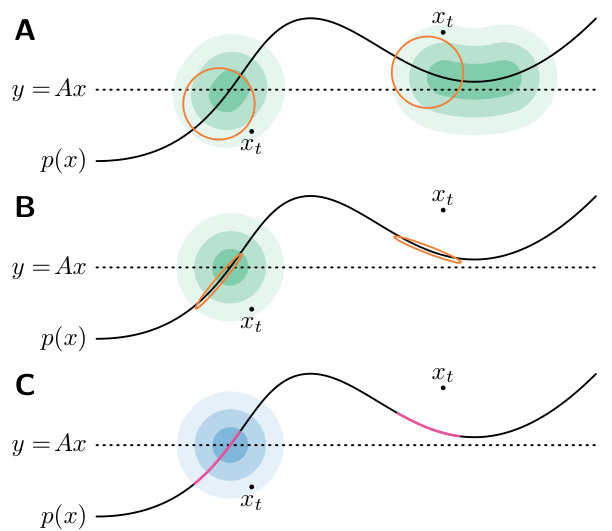
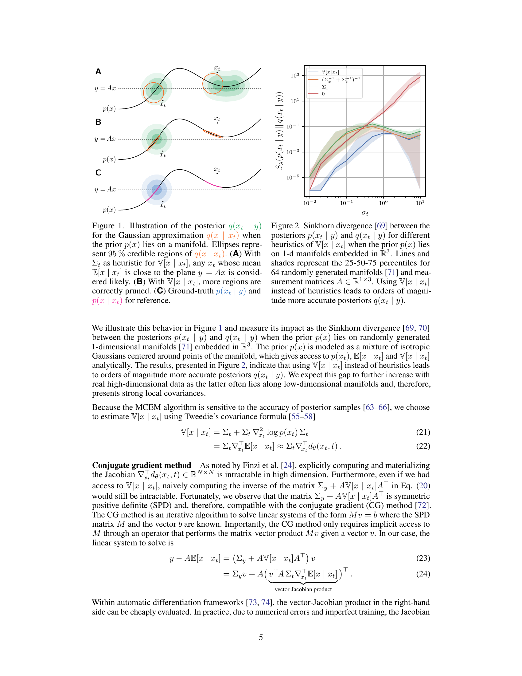
🔼 This figure compares different approximations of the posterior distribution q(xt|y) when the prior p(x) is defined on a manifold. It illustrates how using the true covariance V[x|xt] (panel B) leads to a more accurate posterior estimate compared to using only the mean E[x|xt] (panel A) or simple heuristics like Σt for V[x|xt]. Panel C shows the ground truth posterior for comparison.
read the caption
Figure 1. Illustration of the posterior q(xt | y) for the Gaussian approximation q(x | xt) when the prior p(x) lies on a manifold. Ellipses represent 95% credible regions of q(x | xt). (A) With Et as heuristic for V[x | xt], any xt whose mean E[x | xt] is close to the plane y = Ax is considered likely. (B) With V[x | xt], more regions are correctly pruned. (C) Ground-truth p(xt | y) and p(x | xt) for reference.
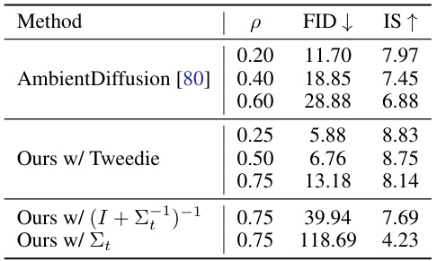
🔼 This table presents the results of evaluating different methods on the corrupted CIFAR-10 dataset. The metrics used are the Fréchet Inception Distance (FID) and the Inception Score (IS), which measure the quality of generated images. Lower FID and higher IS values indicate better image quality. The table shows that the proposed method (‘Ours w/ Tweedie’) outperforms AmbientDiffusion, especially at higher corruption levels. Furthermore, it demonstrates the importance of using the Tweedie’s formula for covariance estimation, as using heuristics leads to significantly poorer results.
read the caption
Table 1. Evaluation of final models trained on corrupted CIFAR-10. Our method outperforms AmbientDiffusion [80] at similar corruption levels. Using heuristics for V[x | xt] instead of Tweedie’s formula greatly decreases the sample quality.
In-depth insights#
Diffusion Priors#
Diffusion models have recently emerged as powerful priors for Bayesian inverse problems, offering a flexible and data-efficient approach. However, training these models effectively often requires substantial amounts of clean, labeled data, which may be scarce in many real-world applications. This limitation necessitates innovative training methods capable of leveraging incomplete or noisy data. The core idea revolves around the use of diffusion processes to model complex probability distributions, effectively capturing uncertainty and enabling efficient inference. Expectation-Maximization (EM) emerges as a suitable algorithm, allowing iterative refinement of the diffusion model parameters based on noisy observations. By alternating between generating posterior samples and updating the diffusion model, this approach overcomes the challenge of data scarcity and makes diffusion models suitable priors in scenarios with limited or noisy datasets. The effectiveness of the method is demonstrated empirically across various inverse problems, validating its practical value and highlighting its potential to enhance the accuracy and robustness of Bayesian inference in data-constrained settings.
EM for DMs#
The application of Expectation-Maximization (EM) to Diffusion Models (DMs) for Bayesian inverse problems presents a novel approach to training DMs with limited data. EM’s iterative nature elegantly addresses the challenge of obtaining latent variable samples, crucial for DM training, from incomplete or noisy observations. The algorithm alternates between generating samples from a posterior distribution (using a modified posterior sampling scheme to improve stability and accuracy) and updating the DM’s parameters to maximize the likelihood of the observed data. This process overcomes the limitations of typical DM training procedures that require vast quantities of clean data. The core innovation lies in the efficient posterior sampling technique, which leverages the properties of DMs to avoid the computational expense of traditional MCMC or importance sampling approaches. The effectiveness of this method is demonstrated empirically, showcasing improvements over previous approaches on low-dimensional, corrupted CIFAR-10, and accelerated MRI datasets.
MMPS Sampling#
The proposed Moment Matching Posterior Sampling (MMPS) method offers a significant advancement in posterior sampling for diffusion models, particularly within Bayesian inverse problems. MMPS directly addresses the limitations of previous methods by explicitly incorporating the covariance of the posterior distribution, leading to more accurate and stable sample generation. Unlike previous approaches that rely on heuristics or approximations for the covariance, MMPS leverages Tweedie’s formula for a precise estimate. While computationally more demanding, the use of conjugate gradient methods mitigates this, making MMPS feasible for high-dimensional applications. The improved accuracy and stability of MMPS translate to higher-quality posterior samples, crucial for successful Bayesian inference and other downstream tasks. This method proves highly effective in scenarios with strong local covariances, outperforming existing techniques and demonstrating superior convergence in the Expectation-Maximization (EM) algorithm used for training diffusion models from limited or noisy data.
Empirical Bayes#
The concept of Empirical Bayes is crucial to this research, offering a solution to the challenge of specifying informative priors in Bayesian inference problems where obtaining sufficient latent variable data is difficult. The core idea is to estimate the prior distribution from the observed data itself, rather than relying on pre-existing assumptions or extensive data. The paper leverages the strength of diffusion models for the prior and uses the Expectation-Maximization (EM) algorithm to refine this prior based on observations, leading to improved posterior sampling quality. This approach effectively addresses the limitations of traditional EB methods, particularly concerning high-dimensional latent spaces and complex data structures for which simpler prior models fail. While the focus is on linear Gaussian forward models, the EM framework offers a potential path towards handling more complex scenarios. The inherent flexibility and high-quality sample generation capabilities of diffusion models are integral to the success of this innovative EB approach.
Future Works#
Future work could explore several promising directions. Extending the methodology to non-linear forward models is crucial for broader applicability, particularly in scientific domains where linear approximations are insufficient. Investigating the impact of different posterior sampling techniques and their computational efficiency would help optimize the EM algorithm’s performance. Exploring the use of alternative prior models, such as normalizing flows, warrants consideration to assess their potential advantages and limitations compared to diffusion models. Finally, a rigorous theoretical analysis of the proposed EM algorithm’s convergence properties and the quality of the learned prior distribution is needed to provide a stronger foundation for the method. Addressing these points will enhance the robustness and impact of this research.
More visual insights#
More on figures
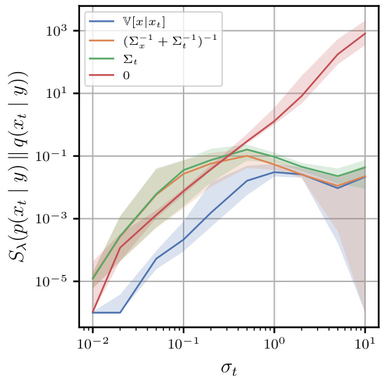
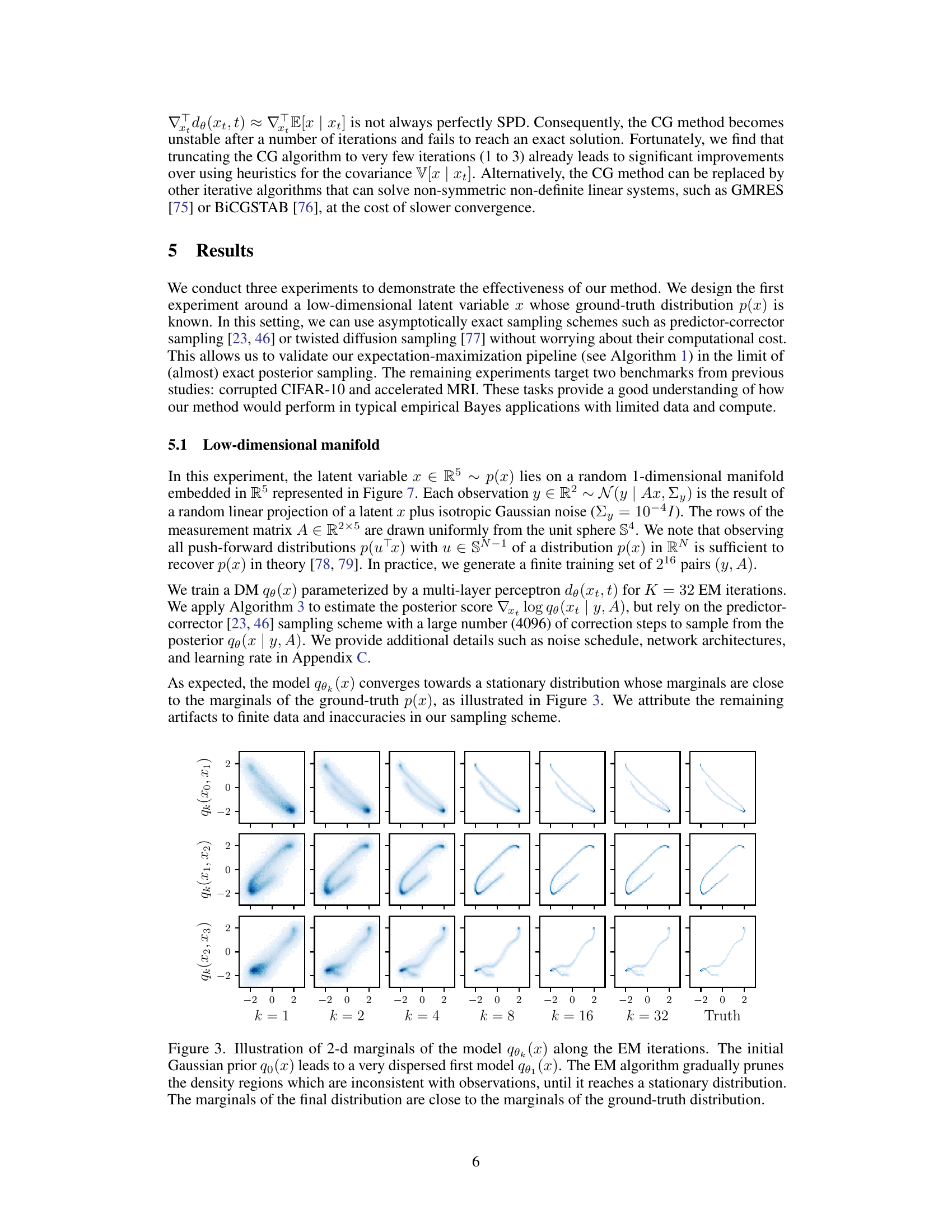
🔼 This figure shows the Sinkhorn divergence between the true posterior distribution and the approximated posterior distribution using different methods for estimating the covariance matrix. It demonstrates that using the exact covariance (V[x|xt]) significantly improves the accuracy of the posterior approximation compared to using heuristics such as Σt or (Σ−1t + Σ−1x)−1. The x-axis represents the diffusion coefficient σt, and the y-axis represents the Sinkhorn divergence.
read the caption
Figure 2. Sinkhorn divergence [69] between the posteriors p(xt | y) and q(xt | y) for different heuristics of V[x | xt] when the prior p(x) lies on 1-d manifolds embedded in R³. Lines and shades represent the 25-50-75 percentiles for 64 randomly generated manifolds [71] and measurement matrices A ∈ R1×3. Using V[x | xt] instead of heuristics leads to orders of magnitude more accurate posteriors q(xt | y).
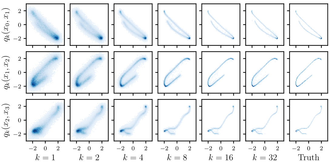
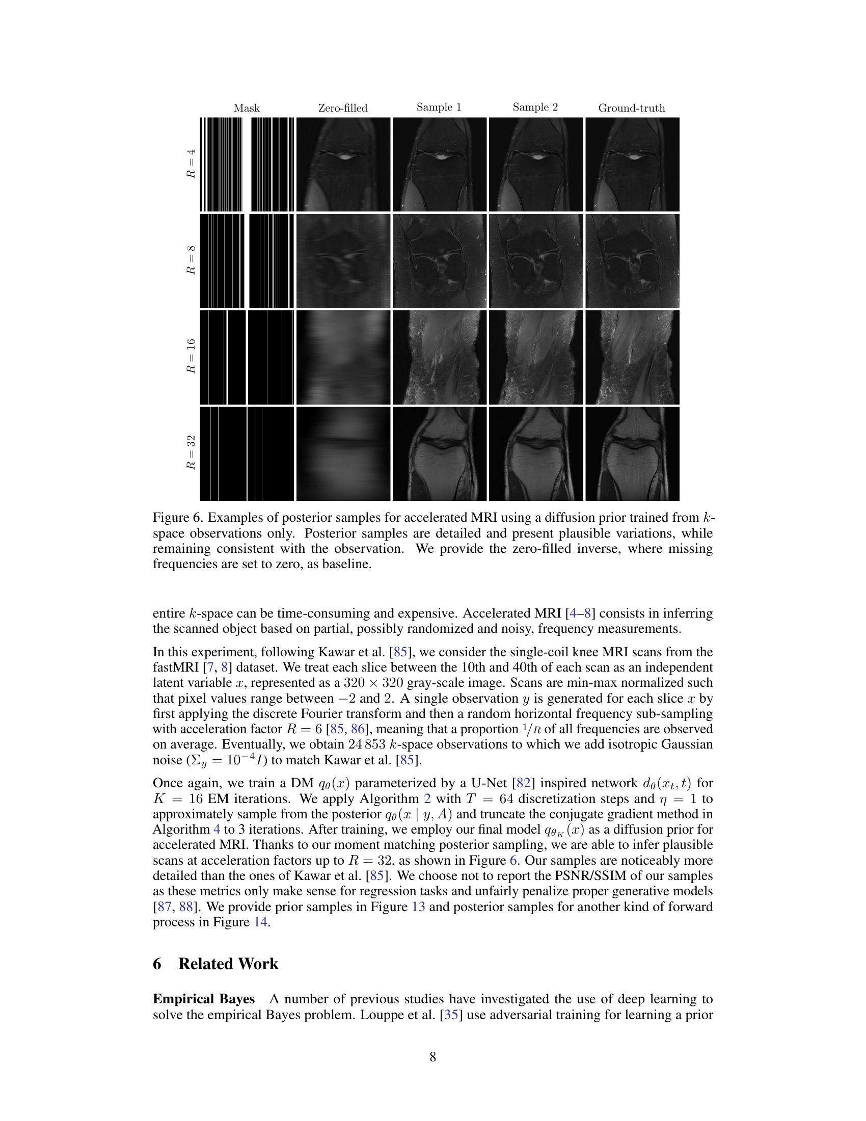
🔼 This figure shows the evolution of the model’s 2D marginals during the Expectation-Maximization (EM) algorithm’s iterations. The initial model is dispersed, but the EM algorithm refines it step by step, improving its consistency with the observations until reaching a stationary distribution resembling the true distribution.
read the caption
Figure 3. Illustration of 2-d marginals of the model qk(x) along the EM iterations. The initial Gaussian prior q0(x) leads to a very dispersed first model q1(x). The EM algorithm gradually prunes the density regions which are inconsistent with observations, until it reaches a stationary distribution. The marginals of the final distribution are close to the marginals of the ground-truth distribution.

🔼 This figure shows the Fréchet Inception Distance (FID) scores over the Expectation-Maximization (EM) iterations for the corrupted CIFAR-10 experiment. Different lines represent different corruption levels (25%, 50%, 75%) and different methods for approximating the posterior covariance (Tweedie’s formula, (I+Σt⁻¹)⁻¹, Σt). The plot illustrates how the FID score (a measure of generated image quality) evolves as the model is trained using the EM algorithm.
read the caption
Figure 4. FID of qθk(x) along the EM iterations for the corrupted CIFAR-10 experiment.

🔼 This figure shows the evolution of the model’s 2D marginal distributions throughout the Expectation-Maximization (EM) algorithm iterations. It starts with a dispersed initial Gaussian prior and gradually refines it by pruning inconsistent regions, converging towards the ground-truth distribution.
read the caption
Figure 3. Illustration of 2-d marginals of the model qk(x) along the EM iterations. The initial Gaussian prior q0(x) leads to a very dispersed first model q1(x). The EM algorithm gradually prunes the density regions which are inconsistent with observations, until it reaches a stationary distribution. The marginals of the final distribution are close to the marginals of the ground-truth distribution.

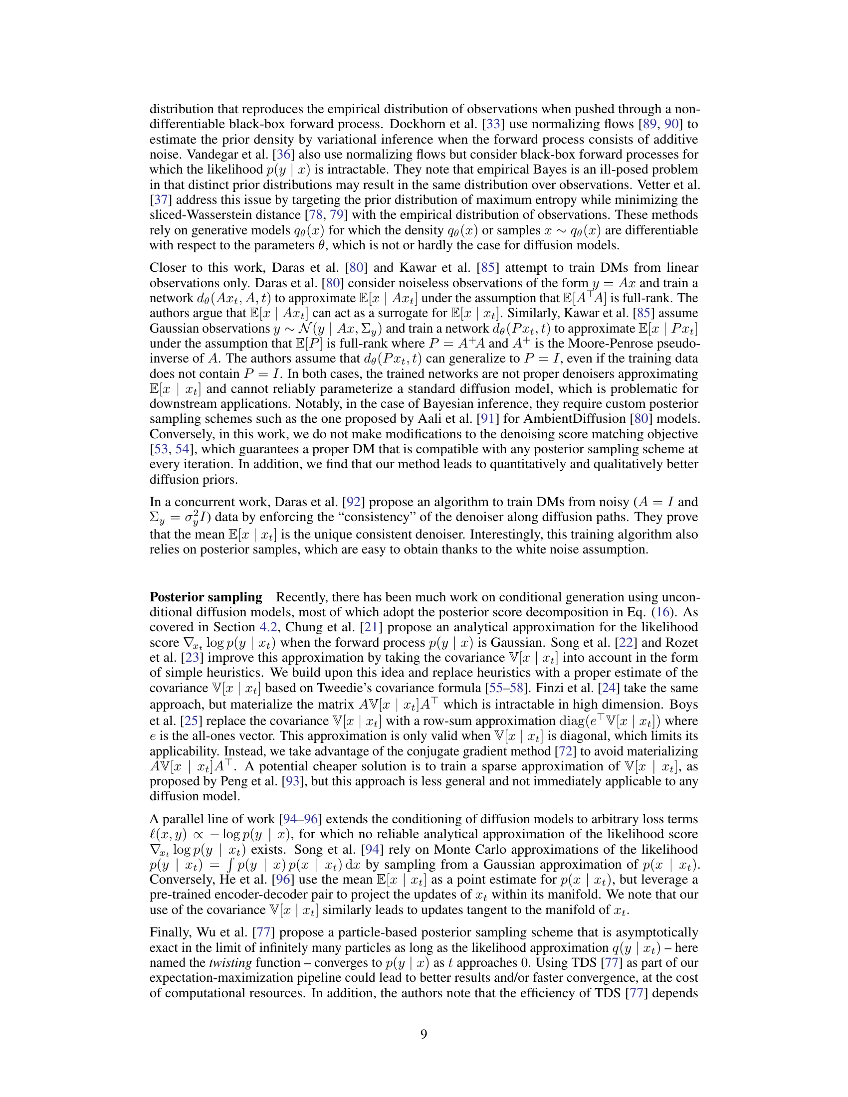
🔼 This figure shows examples of posterior samples generated for accelerated MRI using a diffusion prior. The top row shows the k-space mask, the zero-filled reconstruction (baseline), and two samples generated by the proposed method, along with the ground truth. The figure demonstrates the method’s ability to produce detailed and plausible MRI reconstructions even with missing k-space data.
read the caption
Figure 6. Examples of posterior samples for accelerated MRI using a diffusion prior trained from k-space observations only. Posterior samples are detailed and present plausible variations, while remaining consistent with the observation. We provide the zero-filled inverse, where missing frequencies are set to zero, as baseline.

🔼 This figure shows the 1D and 2D marginal distributions of the ground truth distribution p(x) used in the low-dimensional manifold experiment of the paper. The distribution is defined on a randomly generated 1-dimensional manifold embedded in a 5-dimensional space (R5). The plots visualize the probability density across different dimensions and pairs of dimensions of the latent variable x, illustrating its structure and distribution along the manifold.
read the caption
Figure 7. 1-d and 2-d marginals of the ground-truth distribution p(x) used in the low-dimensional manifold experiment. The distribution lies on a random 1-dimensional manifold embedded in R5.
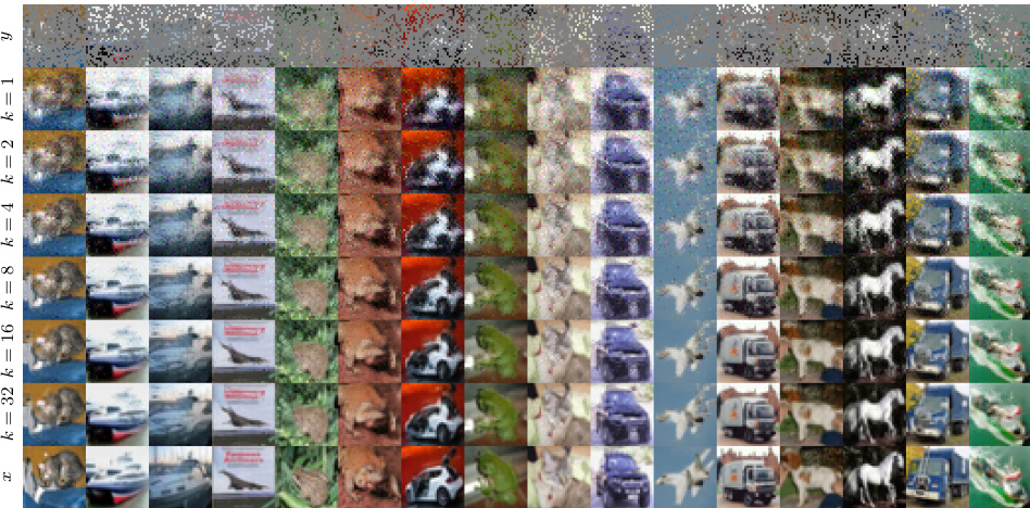
🔼 This figure shows the evolution of the model’s 2D marginal distributions during the Expectation-Maximization (EM) algorithm iterations. The initial Gaussian prior is very broad, but the EM process refines it, gradually focusing on regions consistent with the observed data. The final distribution closely matches the ground truth.
read the caption
Figure 3. Illustration of 2-d marginals of the model qk(x) along the EM iterations. The initial Gaussian prior q0(x) leads to a very dispersed first model q1(x). The EM algorithm gradually prunes the density regions which are inconsistent with observations, until it reaches a stationary distribution. The marginals of the final distribution are close to the marginals of the ground-truth distribution.

🔼 This figure shows the evolution of the learned diffusion model’s marginal distributions across different EM iterations. Starting from a diffuse initial prior, the EM algorithm refines the model by focusing the probability mass onto regions that are consistent with the observed data. The final distribution closely matches the ground truth.
read the caption
Figure 3. Illustration of 2-d marginals of the model qk(x) along the EM iterations. The initial Gaussian prior q0(x) leads to a very dispersed first model q1(x). The EM algorithm gradually prunes the density regions which are inconsistent with observations, until it reaches a stationary distribution. The marginals of the final distribution are close to the marginals of the ground-truth distribution.
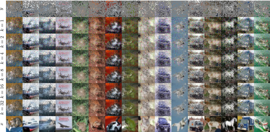
🔼 This figure shows the evolution of the model’s 2D marginal distributions over 32 EM iterations. Starting from a dispersed initial Gaussian prior, the EM algorithm refines the distribution, progressively removing inconsistencies with observed data. The final distribution closely matches the ground truth.
read the caption
Figure 3. Illustration of 2-d marginals of the model qk(x) along the EM iterations. The initial Gaussian prior q0(x) leads to a very dispersed first model q1(x). The EM algorithm gradually prunes the density regions which are inconsistent with observations, until it reaches a stationary distribution. The marginals of the final distribution are close to the marginals of the ground-truth distribution.
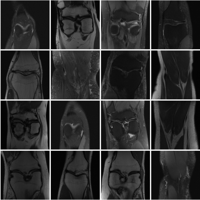
🔼 This figure shows example slices from the fastMRI dataset used in the accelerated MRI experiment of the paper. The images are grayscale and show various knee scans.
read the caption
Figure 11. Example of scan slices from the fastMRI [7, 8] dataset.
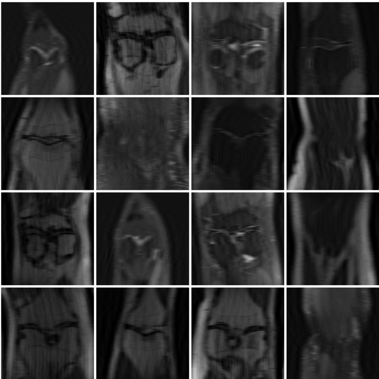
🔼 This figure shows example slices from the fastMRI dataset, which contains knee MRI scans. These images serve as ground truth data for the accelerated MRI experiment described in the paper. The images show the detailed structure and anatomy of the knee.
read the caption
Figure 11. Example of scan slices from the fastMRI [7, 8] dataset.
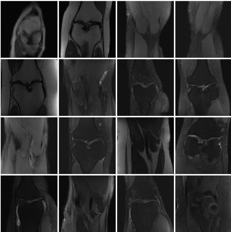
🔼 This figure displays example slices from the fastMRI dataset used in the accelerated MRI experiment of the paper. The images show various knee scans, illustrating the type of data used for training and evaluation of the proposed method.
read the caption
Figure 11. Example of scan slices from the fastMRI [7, 8] dataset.
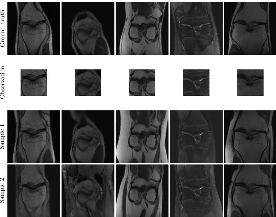
🔼 This figure shows the results of applying the proposed method to the accelerated MRI task. The top row displays the ground truth MRI scans. The second row shows the incomplete k-space observations used as input. The bottom two rows present two different samples from the posterior distribution generated by the model, demonstrating that the model can produce detailed and plausible MRI reconstructions that are consistent with the limited observations. The zero-filled inverse serves as a baseline to compare against, showcasing the improvement achieved by the proposed method.
read the caption
Figure 6. Examples of posterior samples for accelerated MRI using a diffusion prior trained from k-space observations only. Posterior samples are detailed and present plausible variations, while remaining consistent with the observation. We provide the zero-filled inverse, where missing frequencies are set to zero, as baseline.

🔼 This figure shows samples generated after only two Expectation-Maximization (EM) iterations using a specific heuristic for the covariance matrix. The result showcases the negative impact of using less accurate heuristics on the quality of the samples, leading to artifacts (vertical lines). This highlights the importance of the more accurate Tweedie’s formula proposed in the paper.
read the caption
Figure 15. Example of samples from the model qθk (x) after k = 2 EM iterations for the accelerated MRI experiment when the heuristic (I + Σt−1)−1 is used for V[x | xt]. The samples start to present vertical artifacts due to poor sampling.
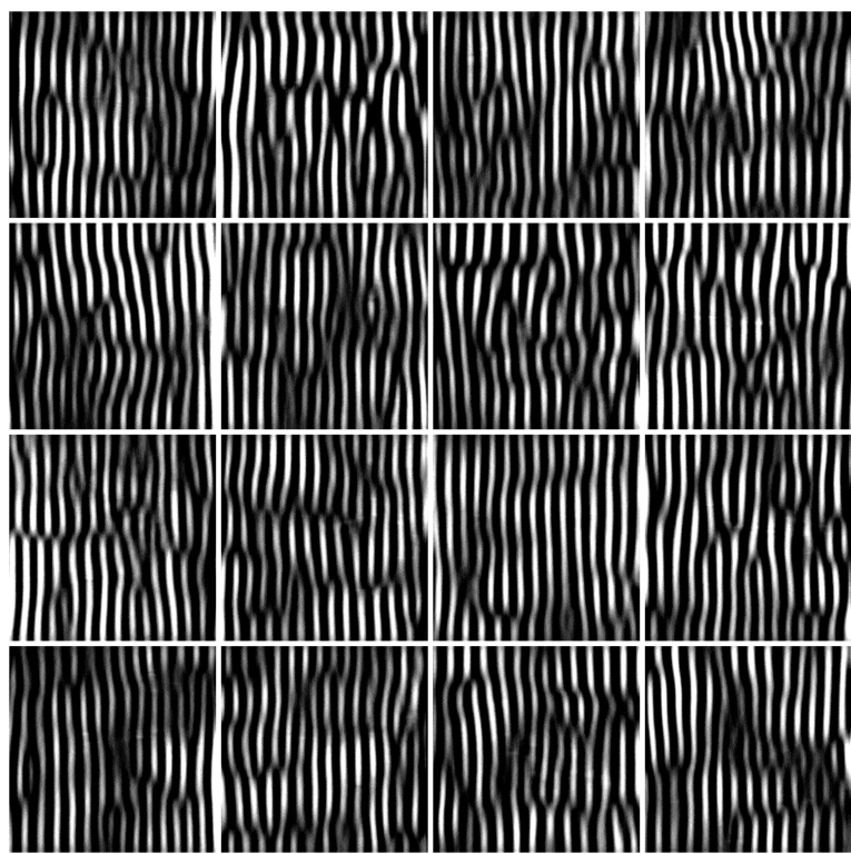
🔼 This figure displays the marginal and 2D marginal distributions of the ground truth data used for the low-dimensional manifold experiment. The data is sampled from a 1-dimensional manifold embedded in 5 dimensions. The plot visually shows the underlying structure of the data used for the experiment.
read the caption
Figure 7. 1-d and 2-d marginals of the ground-truth distribution p(x) used in the low-dimensional manifold experiment. The distribution lies on a random 1-dimensional manifold embedded in R5.
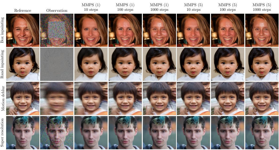
🔼 This figure shows a qualitative comparison of the results obtained using MMPS with 1 and 5 solver iterations for four different inverse problems: box inpainting, random inpainting, motion deblurring, and super-resolution. For each problem, the top row shows the reference image, the second row shows the observation, and subsequent rows display samples generated by MMPS with different numbers of solver iterations (10, 100, and 1000 steps). The figure visually demonstrates the improved image quality achieved by MMPS when increasing the number of solver iterations, particularly for more challenging tasks like motion deblurring.
read the caption
Figure 17. Qualitative evaluation of MMPS with 1 and 5 solver iterations.
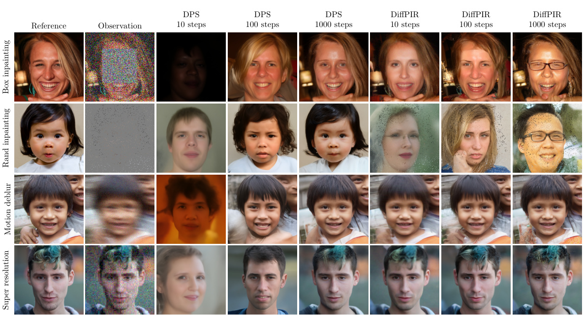
🔼 This figure shows a qualitative comparison of the results obtained by using three different posterior sampling methods: DPS, DiffPIR, and MMPS. For each method, the results obtained with 10, 100, and 1000 sampling steps are shown, for four different image reconstruction tasks: box inpainting, random inpainting, motion deblurring, and super-resolution. By comparing the visual results, one can assess the qualitative performance of each method in generating high-quality images from the noisy or incomplete observations.
read the caption
Figure 18. Qualitative evaluation of DPS [21] and DiffPIR [26].
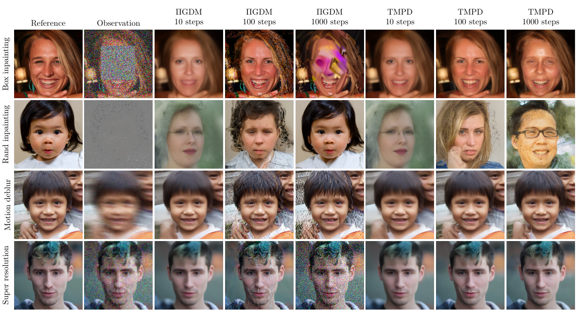
🔼 This figure shows a qualitative comparison of the image reconstruction results obtained using IGDM and TMPD methods for four different inverse problems: box inpainting, random inpainting, motion deblur, and super-resolution. Each row represents a different inverse problem, with the reference image, the noisy observation, and the reconstruction results for IGDM and TMPD, each with different numbers of sampling steps (10, 100, 1000). The figure allows for visual comparison of the quality of image reconstruction achieved by the two different methods under varying noise and degradation conditions.
read the caption
Figure 19. Qualitative evaluation of IGDM [22] and TMPD [25].
More on tables

🔼 This table lists the hyperparameters used in the low-dimensional manifold experiment. It specifies details of the neural network architecture (MLP type, input and hidden layer dimensions, activation function (SiLU), and normalization (LayerNorm)), optimization settings (Adam optimizer, weight decay, learning rate schedule, gradient clipping), batch size, and the number of optimization steps and EM iterations.
read the caption
Table 2. Hyperparameters for the low-dimensional manifold experiment.
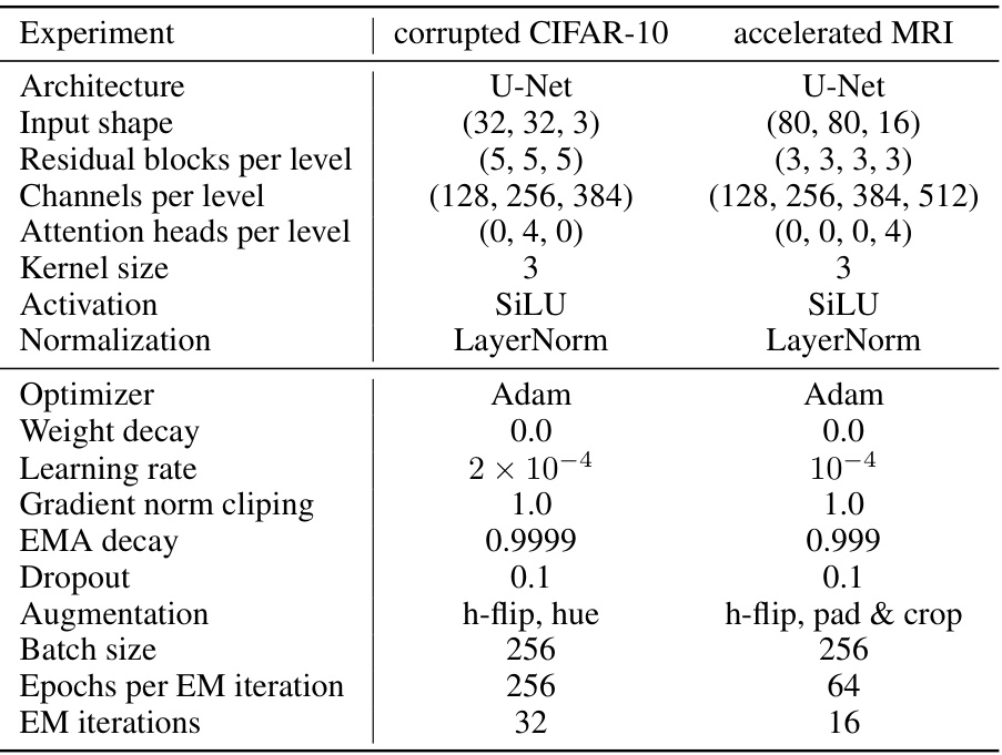
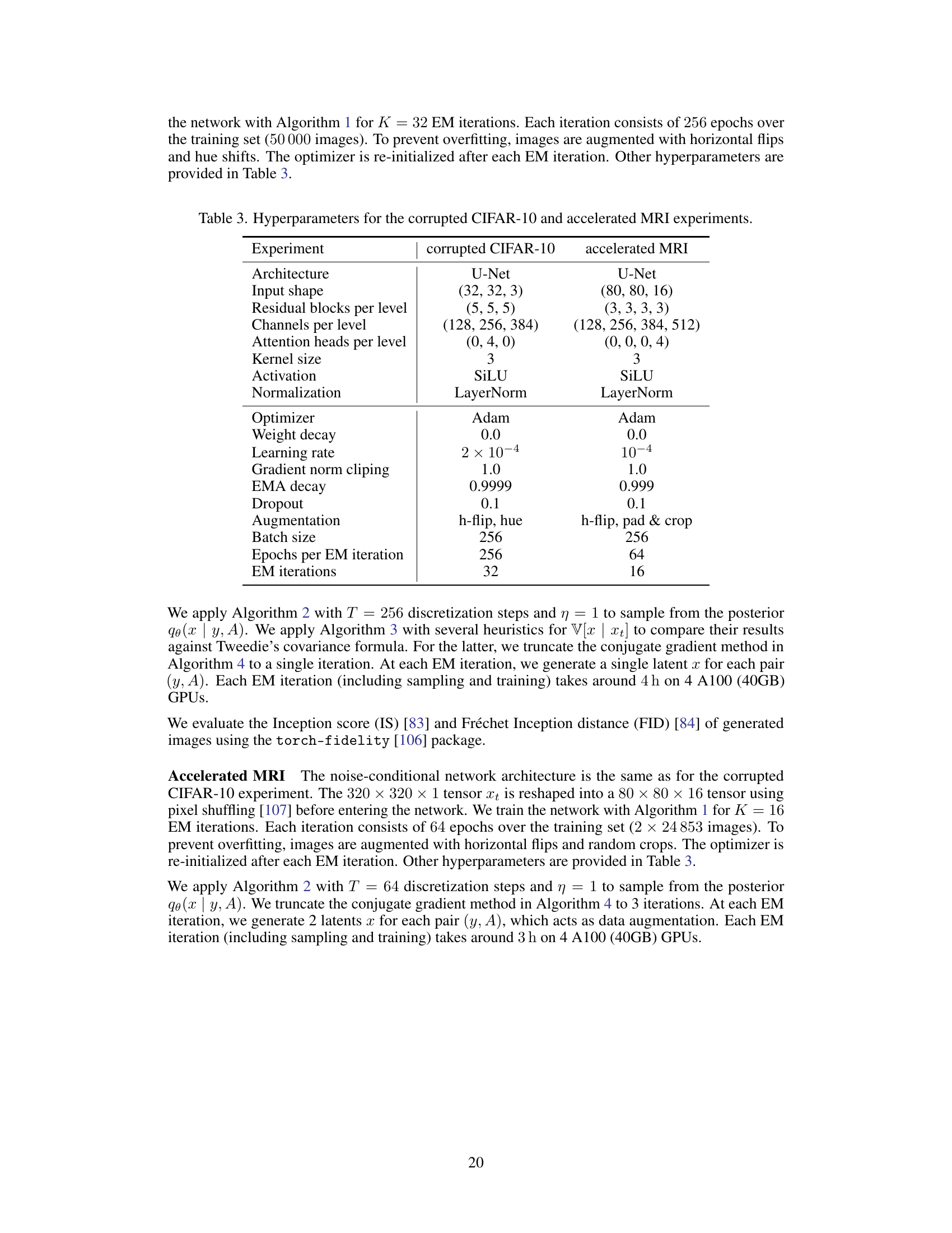
🔼 This table lists the hyperparameters used for the corrupted CIFAR-10 and accelerated MRI experiments. It details the architecture (U-Net for both), input shape, residual blocks per level, channels per level, attention heads per level, kernel size, activation function (SiLU), normalization (LayerNorm), optimizer (Adam), weight decay, learning rate, gradient norm clipping, EMA decay, dropout rate, augmentation techniques, batch size, epochs per EM iteration, and the number of EM iterations. These settings are crucial for reproducibility of the experimental results.
read the caption
Table 3. Hyperparameters for the corrupted CIFAR-10 and accelerated MRI experiments.

🔼 This table presents a quantitative comparison of the Moment Matching Posterior Sampling (MMPS) method against other state-of-the-art posterior sampling methods across four linear inverse problems: box inpainting, random inpainting, motion deblur, and super resolution. The evaluation metrics used are LPIPS, PSNR, and SSIM. The number of solver iterations (1, 3, and 5) for MMPS is also varied to show the impact of increasing computational effort on performance. The results indicate the relative performance of each method across different tasks and solver iterations.
read the caption
Table 4. Quantitative evaluation of MMPS with 1, 3 and 5 solver iterations.
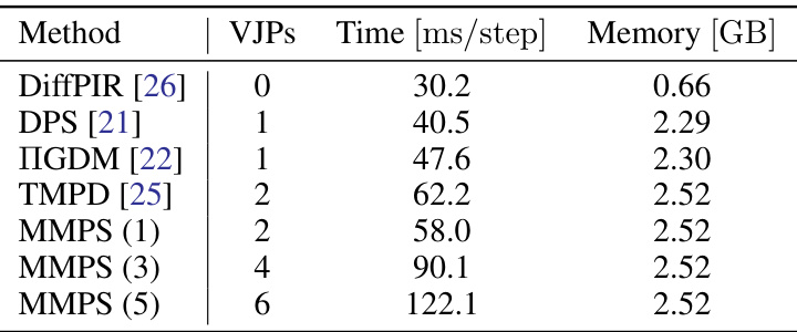
🔼 This table presents the computational cost of the MMPS method compared to other methods for a super-resolution task. It shows the number of vector-Jacobian products (VJPs), time per step, and memory usage for MMPS with varying numbers of solver iterations. The results indicate that while MMPS has a higher computational cost than some baselines, its memory usage is comparable and the increase in time is linear with the number of VJPs.
read the caption
Table 5. Time and memory complexity of MMPS for the 4× super resolution task. Each solver iteration increases the time per step by around 16 ms. The maximum memory allocated by MMPS is about 10% larger than DPS [21] and IGDM [22].
Full paper#
