TL;DR#
Self-supervised learning is crucial for AI due to the high cost of data annotation. Masked Autoencoders (MAE) have shown promise but their learning mechanisms are not fully understood and there’s a drive for improving their training efficiency. Current informed masking techniques often rely on external data sources, undermining the self-supervised nature of MAE.
This research delves into the internal workings of MAE and discovers that it inherently learns patch-level clustering. This understanding leads to the development of ‘Self-guided MAE’, a novel method that generates informed masks based solely on the model’s internal progress in patch clustering. This significantly improves training speed and performance on several downstream tasks, demonstrating the effectiveness of an entirely unsupervised and self-guided approach to improving MAE.
Key Takeaways#
Why does it matter?#
This paper is crucial because it significantly advances self-supervised learning, a critical area in AI. By enhancing the Masked Autoencoder (MAE) model, it offers a more efficient and effective approach to representation learning, thus impacting various downstream tasks. The method is particularly important because it is entirely unsupervised, removing the need for costly data annotation, a significant constraint in modern AI. The findings open up exciting new avenues for research in self-supervised learning and related fields, promising advancements in image processing and beyond.
Visual Insights#

🔼 This figure compares the original MAE with the proposed self-guided MAE. It shows how random masking in the original MAE leads to less distinguishable patch-level clustering, while the self-guided method generates informed masks that accelerate the training process by focusing on less easily separable patches. The figure highlights the improved embedding space achieved with the self-guided method and the superior ability to discern patch-level clustering.
read the caption
Figure 1: Illustration of our self-guided MAE.
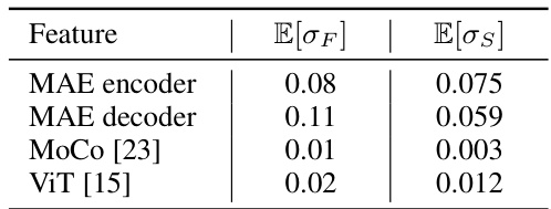
🔼 This table presents a quantitative comparison of feature variance (σF) and similarity variance (σs) for different models: MAE encoder, MAE decoder, MoCo [23], and ViT [15]. Higher values of σF indicate more diverse patch embeddings in the feature space, while higher σs indicates stronger patch clustering. The results demonstrate that MAE encoder and decoder exhibit significantly higher variance compared to MoCo and ViT, indicating superior patch clustering capability.
read the caption
Table 1: Feature variance (σF) and similarity variance (σs).
In-depth insights#
Self-Guided MAE#
The proposed “Self-Guided MAE” method offers a compelling advancement in self-supervised learning. By internally generating informed masks based on the model’s own progress in learning patch-level clustering, it avoids the limitations of relying on external data or pre-trained models. This innovative approach leverages the intrinsic pattern-based clustering ability discovered within vanilla MAE, significantly accelerating the training process. The core idea is to utilize the model’s understanding of image structure, thus eliminating the need for random masking. This makes the learning process more efficient and focused, leading to improved performance on downstream tasks. The method’s unsupervised nature and reliance on internal cues are its strengths, demonstrating the potential of self-guided learning in improving the efficiency of self-supervised approaches. The results suggest substantial improvements in various downstream tasks, making this a promising contribution to the field.
Patch Clustering#
The concept of ‘patch clustering’ in the context of masked autoencoders (MAEs) is crucial. MAE’s success hinges on its ability to learn meaningful representations from masked image patches. The paper investigates how MAE intrinsically performs patch clustering, revealing that it learns pattern-based clusterings surprisingly early in pre-training. This inherent capability is further leveraged by a novel self-guided approach that utilizes internal progress in clustering to generate informed masks. This improves training efficiency by focusing the learning process on less distinguishable patches, thereby accelerating the learning process. The analysis of token relations and the introduction of metrics like exploitation rate give significant insights into this self-learning mechanism. The self-guided approach eliminates the need for external models or information, making it a truly self-supervised enhancement to MAE. This highlights that understanding and utilizing the intrinsic properties of MAEs is a key to improving their performance and efficiency.
Informed Masking#
Informed masking techniques in self-supervised learning aim to enhance the performance of masked autoencoders (MAE) by replacing random masking with more strategic approaches. Instead of randomly masking image patches, informed masking leverages additional information to select which patches to mask, such as attention maps, pre-trained models, or adversarial techniques. This approach is driven by the understanding that selectively masking informative patches can significantly improve model learning and downstream task performance. However, a key challenge is the reliance on external resources or pre-trained models, limiting the purely self-supervised nature of the initial MAE framework. The effectiveness of informed masking hinges on the quality of the information used to guide the masking process. High-quality information leads to superior performance gains, whereas noisy or irrelevant information may hinder learning or even degrade performance compared to standard random masking. Future research should focus on developing novel, purely self-supervised methods for informed masking that eliminate the need for external data or models while effectively improving MAE’s learning capabilities.
Early Clustering#
The concept of ‘Early Clustering’ in the context of self-supervised learning models, specifically masked autoencoders (MAEs), suggests that the model begins to form meaningful groupings of image patches surprisingly early in the training process. This contradicts the naive assumption that such semantic understanding only emerges after extensive training. The early formation of these clusters implies that the model isn’t merely learning low-level features but rather starts to organize the data in a way that reflects higher-level relationships. This early clustering phenomenon is significant because it provides insights into how MAEs learn, highlighting the role of patch-level relationships and the potential for improving their training efficiency by building upon this intrinsic behavior. Understanding when and how this early clustering emerges is crucial for optimizing the training process of MAEs. Further research could leverage this knowledge to develop more efficient informed masking strategies, which intelligently guide the model’s attention and accelerate the development of higher-level representations.
Decoder Analysis#
A thorough decoder analysis in a research paper would involve investigating its internal mechanisms and how it interacts with other components, particularly the encoder. Key aspects would include exploring the decoder’s architecture, focusing on its layers, activation functions, and the role of mask tokens. Understanding how the decoder reconstructs the masked parts of the input is crucial, examining if it leverages contextual information from the visible parts or employs any specific strategies for pattern completion or feature synthesis. A quantitative analysis might involve calculating reconstruction error metrics across different masking ratios or comparing the decoder’s performance to various baselines. Analyzing the decoder’s learned representations to check for clustering or other meaningful structures in its feature space and investigating if the decoder’s learning dynamics correlate with the encoder’s learning process are valuable. The relationship between the quality of the decoder’s output and the effectiveness of the overall model for downstream tasks would be a key aspect of the analysis, determining if the decoder’s performance is a bottleneck or a contributing factor to the model’s overall success.
More visual insights#
More on figures
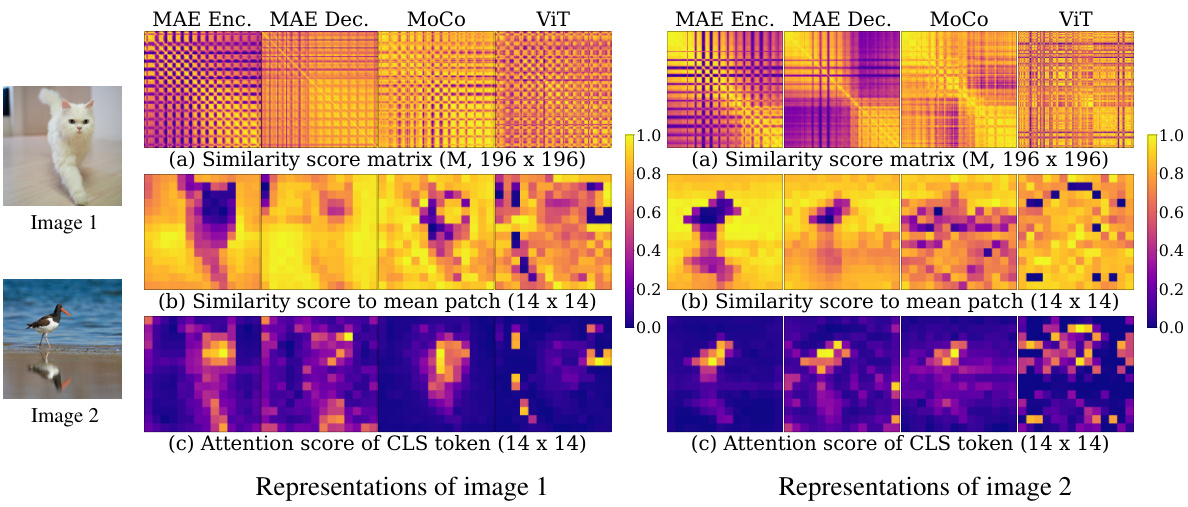
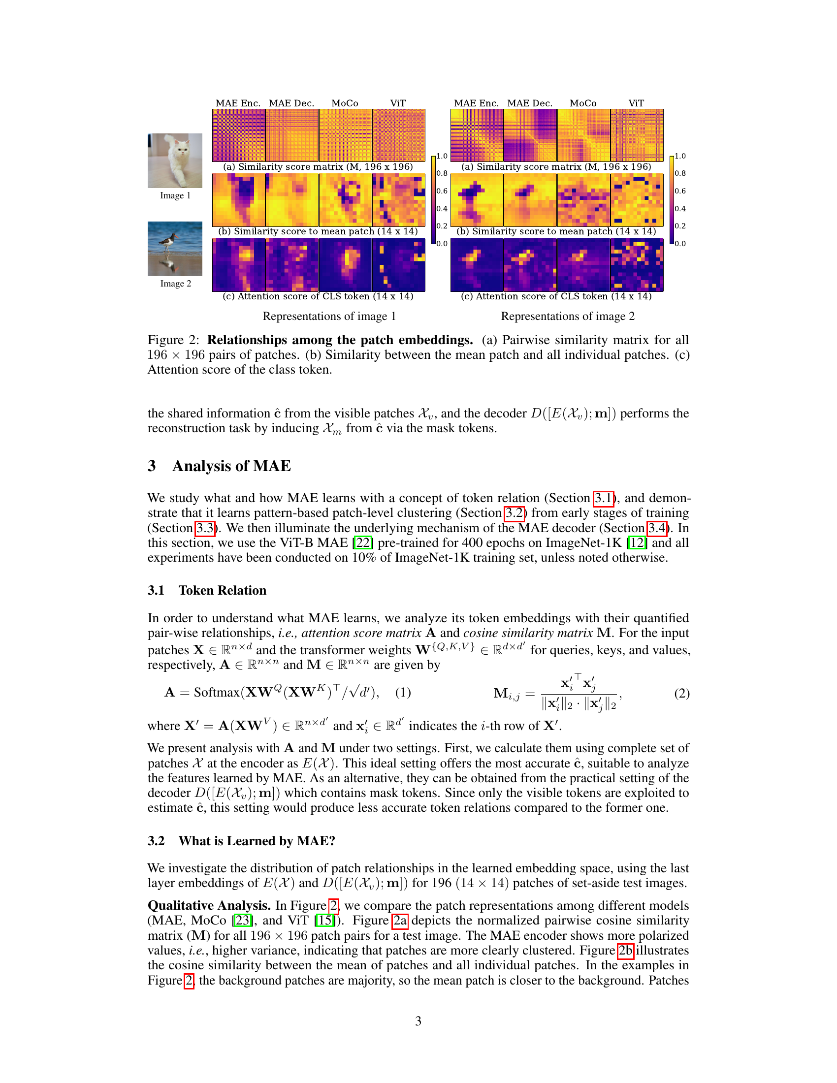
🔼 This figure compares the patch relationships in the learned embedding space, using the last layer embeddings for 196 (14 × 14) patches of test images. The analysis includes a pairwise similarity matrix (M) showing the relationships between all pairs of patches, a similarity score showing the relationship between each patch and the average patch, and the attention score of the class (CLS) token. The visualizations highlight how the MAE encoder shows more polarized values indicating clear patch clustering compared to MoCo and ViT.
read the caption
Figure 2: Relationships among the patch embeddings. (a) Pairwise similarity matrix for all 196 × 196 pairs of patches. (b) Similarity between the mean patch and all individual patches. (c) Attention score of the class token.

🔼 This figure shows that the MAE model starts learning patch clustering from the very early stage of training. The left graph (a) illustrates how the gap between the mean intra-cluster edge weights and the mean inter-cluster edge weights increases over training epochs. This indicates that the model is progressively learning to better distinguish between different clusters of patches. The right graph (b) shows how the KL divergence between the distribution of token relations at different training epochs and the final converged distribution decreases rapidly at early epochs and then gradually levels off. This confirms that token relations converge early in the training process and that patch clustering is learned from the beginning of the training process. The numbers in the legend of graph (b) specify the layer number of MAE. Appendix B contains more details.
read the caption
Figure 3: MAE learns patch clustering from very early stage of training process. (a) MAE widens the gap µintra − µinter. (b) Token relations drastically converge at early epochs and then gradually level off. Numbers in the legend denote the layer i. More details are provided in Appendix B.

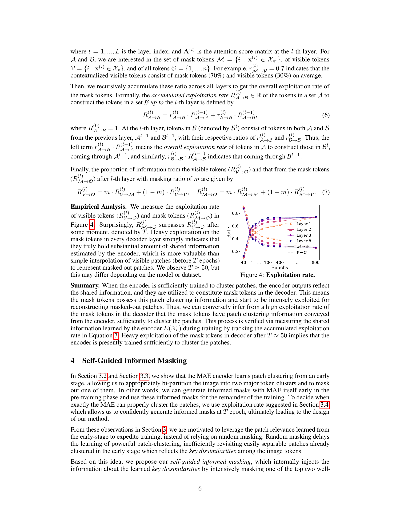
🔼 This figure shows the exploitation rate of visible tokens (R(L)V→O) and mask tokens (R(L)M→O) in each decoder layer. The exploitation rate is a measure of how much the mask tokens are used to reconstruct the masked-out patches. The figure shows that the exploitation rate of mask tokens surpasses that of visible tokens after around 50 epochs. This suggests that the decoder is able to leverage the information learned by the encoder from the visible tokens to reconstruct the masked-out tokens.
read the caption
Figure 4: Exploitation rate.
🔼 This figure compares the original MAE with the proposed self-guided MAE. The original MAE uses random masking, while the self-guided MAE generates informed masks covering the main object entirely. The informed masks are generated using distinguishable patch representations that emerge early in the training process. This leads to faster training and clearer embeddings. The figure shows the input image, random masking, MAE feature, bi-partitioned masking, informed masking with a hint, and the proposed method’s feature.
read the caption
Figure 1: Illustration of our self-guided MAE.
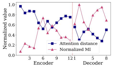
🔼 This figure shows two plots: attention distance and normalized mutual information (NMI) across different layers of the MAE model. The attention distance measures how globally each layer attends to the image while NMI measures the homogeneity of the attention map. The plots show that the attention distance increases and NMI increases up to a certain point, and then they decrease in the decoder layers. This indicates that the early layers of the encoder tend to attend to more local regions, while the later layers attend to the entire image. The decoder shows a similar trend, but the values are lower.
read the caption
Figure 6: MAE properties.

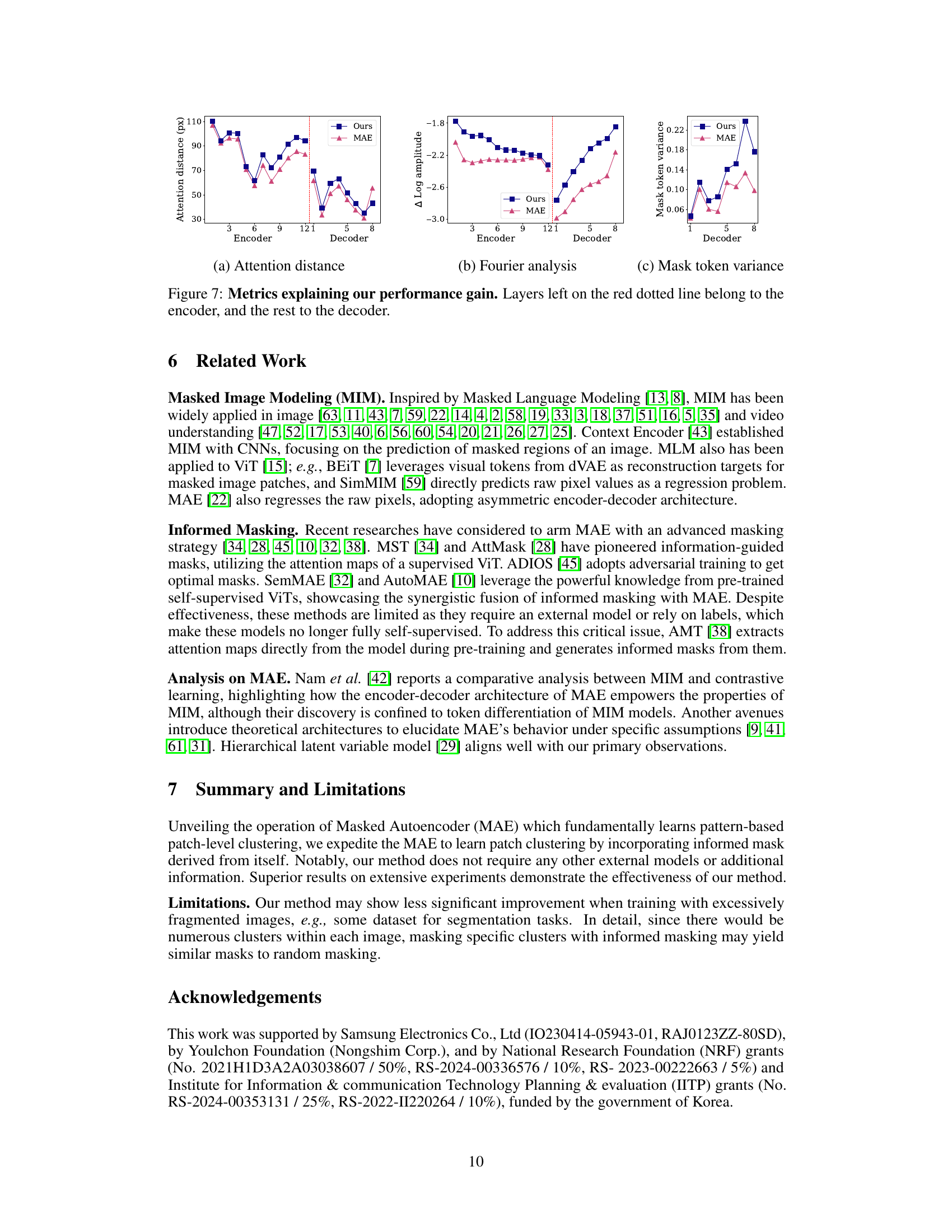
🔼 This figure shows three subfigures that analyze the learned feature space of the proposed method and compares it to the vanilla MAE. Subfigure (a) displays the attention distance, showing how well the model captures global image context. Subfigure (b) presents a Fourier analysis of the learned features, highlighting the emphasis on high-frequency components (patterns). Subfigure (c) illustrates the variance of mask token embeddings in decoder layers, reflecting the diversity of learned patch clusters. The results indicate that the proposed method learns more global features, emphasizes pattern-based representation, and achieves finer patch-level clustering compared to the vanilla MAE.
read the caption
Figure 7: Metrics explaining our performance gain. Layers left on the red dotted line belong to the encoder, and the rest to the decoder.

🔼 This figure illustrates the hierarchical latent variable model framework of Masked Autoencoders. It shows how the encoder estimates high-level latent variables (shared information) from visible patches to reconstruct masked-out patches. The dotted line represents the potential statistical dependency between visible and masked patches. It visually explains the process of reconstructing masked-out image information by leveraging the learned high-level latent variables representing the entire image.
read the caption
Figure I: Hierarchical latent variable model framework [29]. Assuming high-level shared information c exists among the whole tokens, MAE encoder learns to estimate ĉ from X to reconstruct raw pixels of Xm. Here, shared information is equivalent to statistical dependency inside X. sm and sv stand for information specific to Xm and Xu, respectively. Dotted line indicates potential dependency.
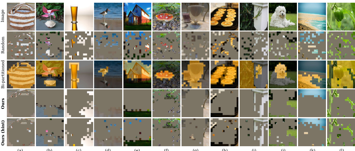
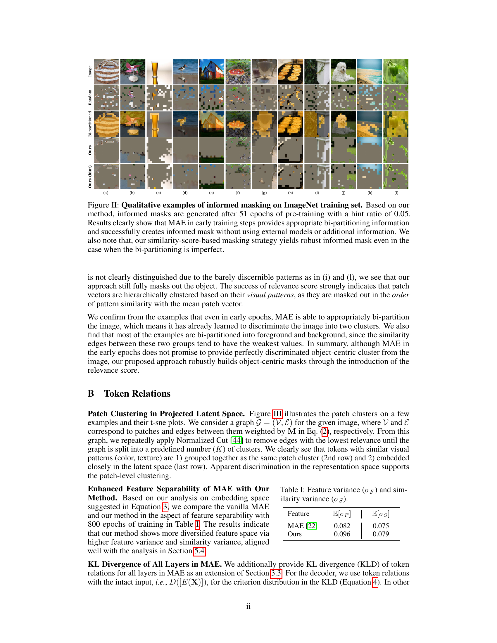
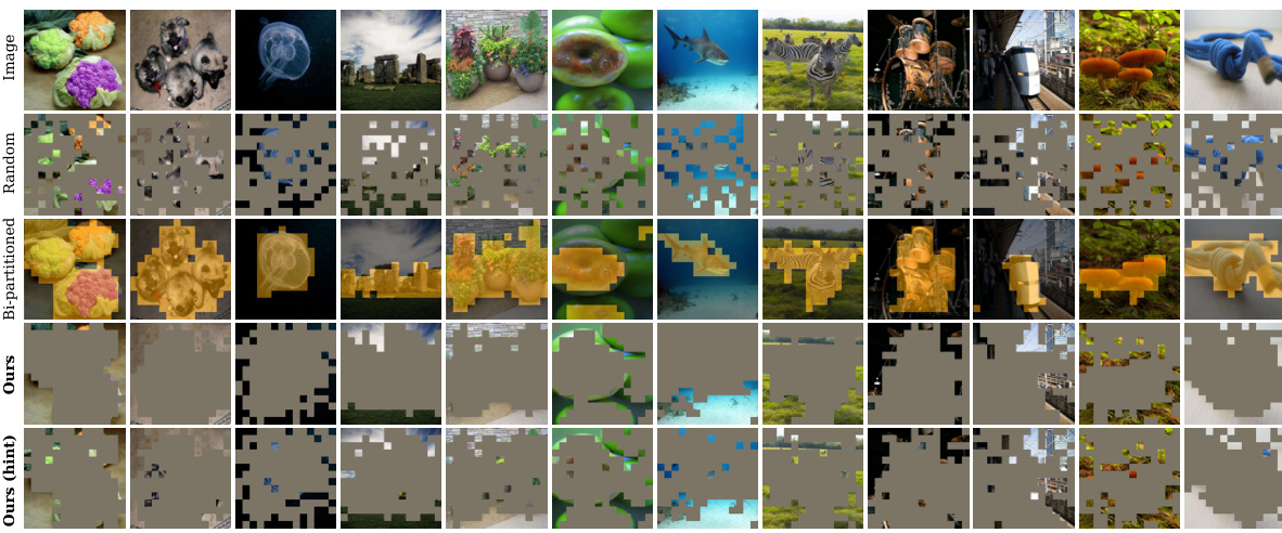
🔼 This figure provides several examples to visually compare different masking strategies. The top row shows the input images. The second row shows the images after random masking. The third row shows the images after bi-partitioned masking. The fourth row displays the images after applying the proposed self-guided informed masking method. The bottom row shows the result of the proposed method with hint tokens added. The figure demonstrates how the proposed method generates more informative masks by focusing on the main object in each image, leading to improved performance in downstream tasks.
read the caption
Figure 5: Examples of Self-guided Informed masking. More examples and detailed explanations on our method are displayed in Appendix A.

🔼 This figure shows examples of patch clustering learned by the MAE model. It contains three rows. The top row (a) shows example input images. The middle row (b) shows the images again, but with patches colored according to which cluster they belong to, illustrating that MAE groups similar patches (e.g., similar textures or colors) together. The bottom row (c) uses t-SNE to project the patch embeddings into a 2D space, visually demonstrating that patches assigned to the same cluster are located near each other in the embedding space. The figure visually demonstrates the ability of MAE to learn patch-level clustering from raw image data.
read the caption
Figure III: Illustrations of patch clusters learned by MAE. (a) Input images. (b) Similarity-based patch clusters. (c) t-sne plots of the patch embeddings.
🔼 This figure shows that MAE starts learning patch-level clustering from the very beginning of pre-training. Part (a) tracks the difference between the mean intra-cluster and mean inter-cluster edge weights over training epochs, showing a widening gap indicating increasing clustering. Part (b) shows the KL divergence of token relations over epochs for different layers, illustrating that relations converge rapidly in early epochs and then stabilize, indicating early establishment of patch clusters.
read the caption
Figure 3: MAE learns patch clustering from very early stage of training process. (a) MAE widens the gap μintra−μinter. (b) Token relations drastically converge at early epochs and then gradually level off. Numbers in the legend denote the layer i. More details are provided in Appendix B.

🔼 This figure compares the performance of three different models (MAE, MoCo, and ViT) in terms of bi-partitioning image patches into two clusters. It shows how the gap between the mean intra-cluster and inter-cluster similarity scores changes over training epochs using two different metrics: similarity score and attention score. The plots illustrate that MAE consistently widens the gap, indicating effective patch clustering, whereas MoCo shows a clear gap from early stages, and ViT exhibits inconsistent behavior. This visualization supports the paper’s claim that MAE excels at learning pattern-based patch-level clustering.
read the caption
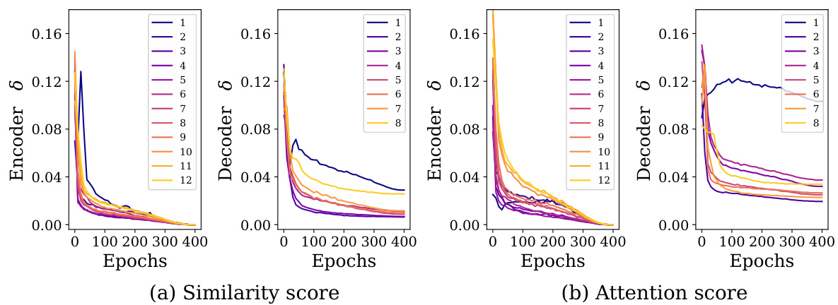
Figure V: Bi-partitioning performance of various models. MAE, MoCo and ViT show different trends of bi-partitioning performance in both of (a) similarity score and (b) attention score.

🔼 This figure shows that MAE learns patch clustering from a very early stage of training. The first graph (a) shows the difference between intra-cluster and inter-cluster edge weights over training epochs using both cosine similarity and attention scores; this gap increases over time, demonstrating the separation of clusters. The second graph (b) displays the KL divergence of token relations across training epochs for different layers; it demonstrates rapid convergence at early stages, signifying the establishment of patch-level clustering relationships early in the training process.
read the caption
Figure 3: MAE learns patch clustering from very early stage of training process. (a) MAE widens the gap \(\mu_{intra} - \mu_{inter}\). (b) Token relations drastically converge at early epochs and then gradually level off. Numbers in the legend denote the layer i. More details are provided in Appendix B.

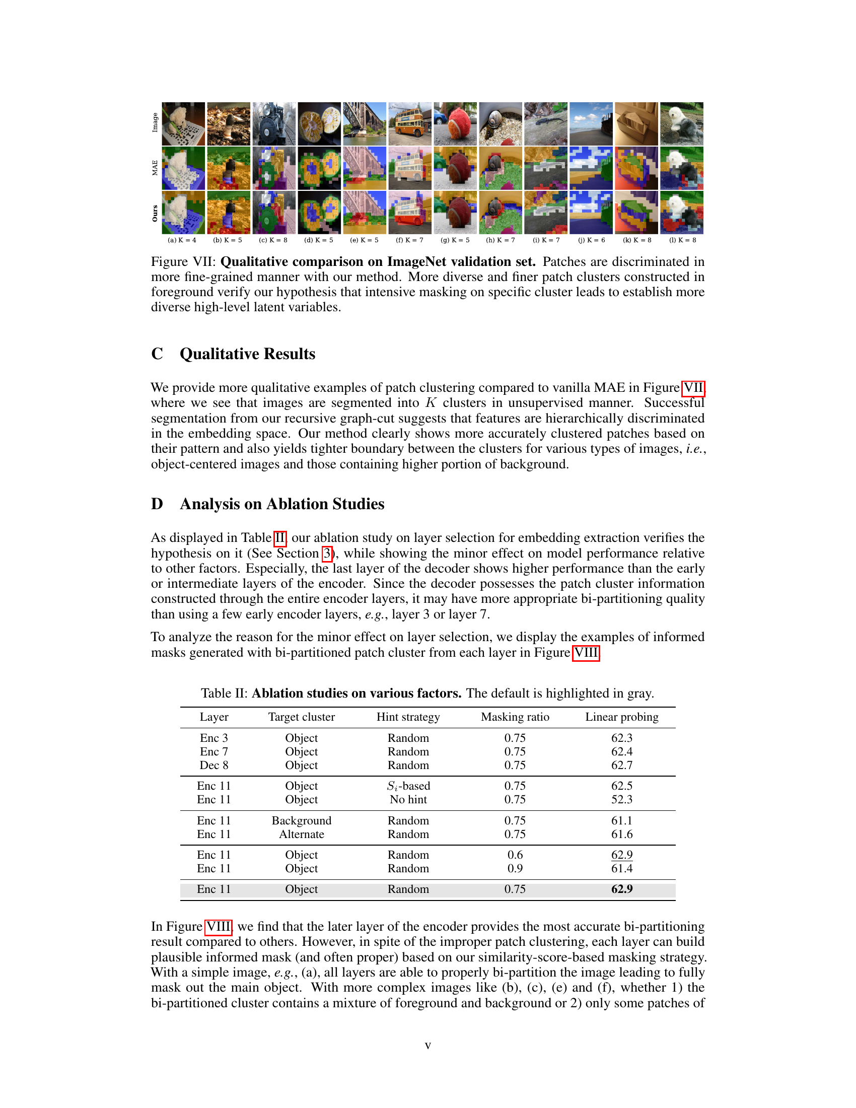
🔼 This figure shows a qualitative comparison of patch clustering between the proposed method and the original MAE on the ImageNet validation set. The top row displays the input images. The middle row shows the patch clustering results obtained using the original MAE. The bottom row displays the patch clustering results obtained using the proposed self-guided masked autoencoder. The figure demonstrates that the proposed method achieves more fine-grained and diverse patch clustering compared to the original MAE, supporting the hypothesis that intensive masking on specific clusters leads to a more diverse set of high-level latent variables. The various colors represent different clusters.
read the caption
Figure VII: Qualitative comparison on ImageNet validation set. Patches are discriminated in more fine-grained manner with our method. More diverse and finer patch clusters constructed in foreground verify our hypothesis that intensive masking on specific cluster leads to establish more diverse high-level latent variables.
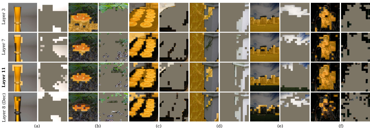
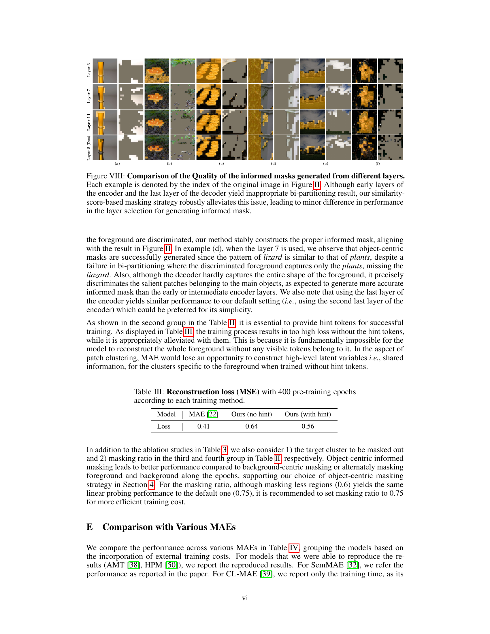
🔼 This figure shows a comparison of the quality of informed masks generated using different layers (Layer 3, Layer 7, Layer 11, and Layer 8 (Decoder)) of the MAE model. The results demonstrate that even though earlier layers of the encoder and the last decoder layer may produce less effective bi-partitioning of images, the similarity-score-based masking method consistently generates good informed masks, minimizing the impact of layer choice on performance.
read the caption
Figure VIII: Comparison of the Quality of the informed masks generated from different layers. Each example is denoted by the index of the original image in Figure II. Although early layers of the encoder and the last layer of the decoder yield inappropriate bi-partitioning result, our similarity-score-based masking strategy robustly alleviates this issue, leading to minor difference in performance in the layer selection for generating informed mask.
More on tables

🔼 This table presents the performance comparison of the proposed method against baseline methods (MAE and AMT) across three downstream tasks: image classification, object detection, and semantic segmentation. For image classification, performance is measured using linear probing (LP) and fine-tuning (FT) on four datasets (ImageNet-1K, iNaturalist 2019, CIFAR, and CUB). Object detection performance is evaluated using average precision for bounding boxes (APbox) and segmentation masks (Apmask) on the COCO dataset. Finally, semantic segmentation performance is measured using mean Intersection over Union (mIoU) on the ADE20K dataset.
read the caption
Table 2: Performance on downstream tasks. LP and FT stand for Linear probing and Fine-tuning, respectively. Det. indicates the Object Detection task.

🔼 This table presents the results of ablation studies conducted to analyze the impact of different factors on the performance of the proposed self-guided masked autoencoder. The studies investigated the choice of layer for embedding extraction, hint strategy, and masking ratio. The results show the linear probing performance for image classification on the ImageNet-1K dataset for each configuration. The default configuration is highlighted in gray, and a more detailed analysis is available in Appendix D.
read the caption
Table 3: Ablation studies. The default is highlighted in gray. Detailed analysis can be found in Appendix D.

🔼 This table presents a quantitative analysis comparing the feature variance (σF) and similarity variance (σs) for different models: MAE encoder, MAE decoder, MoCo, and ViT. Feature variance measures the spread of patch embeddings in the feature space, while similarity variance indicates the strength of patch clustering. Higher values for both indicate more diverse and clearly clustered embeddings. The table shows that MAE (both encoder and decoder) exhibits significantly higher values in both metrics compared to MoCo and ViT, suggesting more effective patch clustering based on visual patterns.
read the caption
Table 1: Feature variance (σF) and similarity variance (σs).

🔼 This table presents the results of ablation studies conducted to evaluate the impact of different factors on the linear probing performance of the proposed self-guided masked autoencoder method for image classification. The studies systematically varied the layer used for embedding extraction, the strategy for generating hint tokens (random or based on similarity score), and the masking ratio. The results show the importance of choosing the appropriate layer, the contribution of hint tokens, and the effect of the masking ratio on the model’s performance.
read the caption
Table 3: Ablation studies. The default is highlighted in gray. Detailed analysis can be found in Appendix D.

🔼 This table presents a comparison of the reconstruction loss (measured as Mean Squared Error or MSE) achieved by three different models after 400 epochs of pre-training. The models compared are the original Masked Autoencoder (MAE), the proposed method without hint tokens, and the proposed method with hint tokens. The table shows that the inclusion of hint tokens in the proposed method significantly reduces reconstruction loss compared to the no hint version, and provides better results than the MAE.
read the caption
Table III: Reconstruction loss (MSE) with 400 pre-training epochs according to each training method.

🔼 This table presents the performance comparison of different models on three downstream tasks: image classification, object detection, and semantic segmentation. The results are given for both linear probing (LP) and fine-tuning (FT) methods. For image classification, multiple datasets (ImageNet-1K, iNat2019, CIFAR, CUB) were used. Object detection results are shown for the COCO dataset and semantic segmentation results for ADE20K. The metrics reported vary based on the task (e.g., accuracy for image classification, APbox and Apmask for object detection, mIoU for semantic segmentation).
read the caption
Table 2: Performance on downstream tasks. LP and FT stand for Linear probing and Fine-tuning, respectively. Det. indicates the Object Detection task.

🔼 This table presents the performance comparison of different models on various downstream tasks, namely image classification, object detection, and semantic segmentation. It shows the results using linear probing (LP) and fine-tuning (FT) methods across several datasets. The metrics used include linear probing accuracy and fine-tuning accuracy for image classification; average precision (AP) for bounding boxes (Apbox) and segmentation masks (Apmask) for object detection; and mean Intersection over Union (mIoU) for semantic segmentation. This allows for a comprehensive evaluation of the model’s ability to transfer learned representations to diverse vision tasks.
read the caption
Table 2: Performance on downstream tasks. LP and FT stand for Linear probing and Fine-tuning, respectively. Det. indicates the Object Detection task.
Full paper#
