Provably and Practically Efficient Adversarial Imitation Learning with General Function Approximation

↗ arXiv ↗ Hugging Face

TL;DR

#

Key Takeaways

#

Why does it matter?

#

This paper is crucial because it bridges the theory-practice gap in adversarial imitation learning. It introduces OPT-AIL, a provably efficient algorithm for general function approximation, a significant advancement over existing methods limited to simplified scenarios. This opens new avenues for research and practical applications in various real-world sequential decision-making tasks.

Visual Insights

#

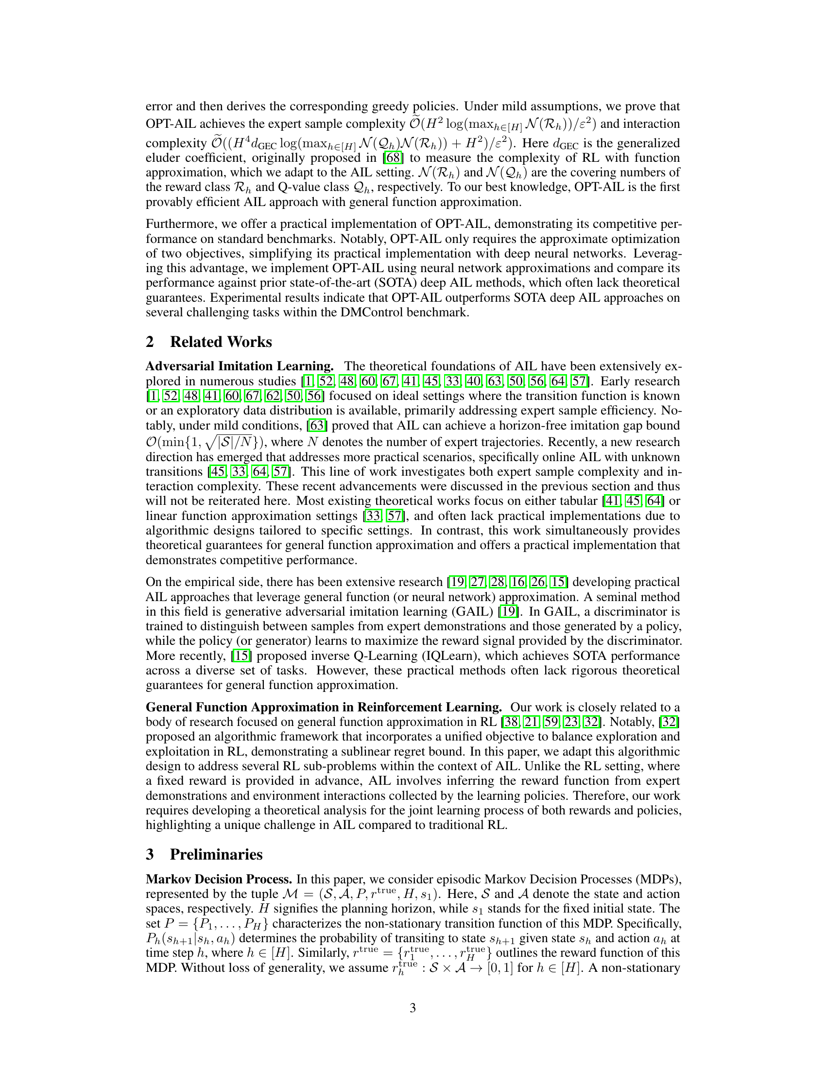
🔼 This figure presents the overall performance comparison of different imitation learning algorithms across eight DMControl tasks. Each algorithm’s performance is evaluated using the average return over 500,000 interactions with the environment. The x-axis indicates the number of expert trajectories used for training, while the y-axis represents the average return achieved. The solid lines show the average return, and the shaded area represents the standard deviation across five independent trials with different random seeds. This figure highlights the relative performance of each algorithm in terms of sample efficiency (how well they perform with a limited number of expert demonstrations).

read the caption

Figure 1: Overall performance on 8 DMControl tasks over 5 random seeds following 500k interactions with the environment. Here the x-axis is the number of expert trajectories and the y-axis is the return. The solid lines are the mean of results while the shaded region corresponds to the standard deviation over 5 random seeds. Same as the following figures.

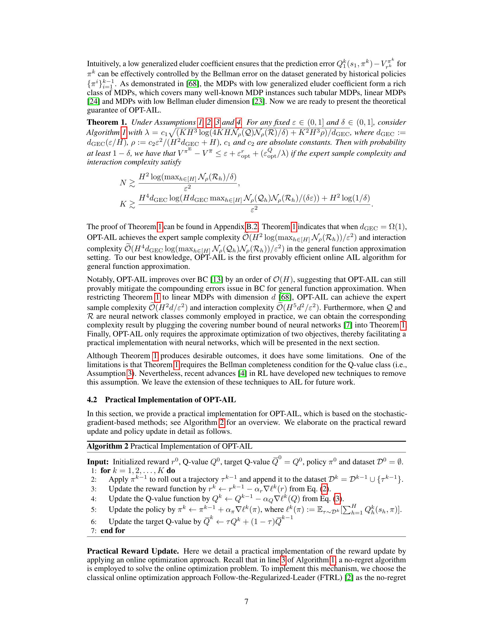
🔼 This table summarizes the expert sample complexity and interaction complexity of several imitation learning algorithms under different settings. The settings include tabular Markov Decision Processes (MDPs), linear mixture MDPs, and MDPs with general function approximation. The algorithms are behavioral cloning (BC), optimization-based adversarial imitation learning (OAL), modified Bayesian adversarial imitation learning (MB-TAIL), optimism-guided adversarial imitation learning (OGAIL), Bellman residual guided imitation learning (BRIG), and the proposed optimization-based adversarial imitation learning (OPT-AIL). The table shows the complexity results in big O notation, highlighting the dependence on the horizon length (H), the desired imitation gap (ɛ), state and action space sizes (|S|, |A|), policy class size (|Π|), feature dimension (d), and generalized eluder coefficient (dGEC).

read the caption

Table 1: A summary of the expert sample complexity and interaction complexity. Here H is the horizon length, ɛ is the desired imitation gap, |S| is the state space size, |A| is the action space size, |Π| is the cardinality of the finite policy class Π, d is the dimension of the feature space, dGEC is the generalized eluder coefficient, N(R_h) and N(Q_h) are the covering numbers of the reward class R_h and Q-value class Q_h, respectively. We use Õ to hide logarithmic factors.

In-depth insights

#

OPT-AIL Algorithm

#

The OPT-AIL algorithm is presented as a novel approach to adversarial imitation learning (AIL), aiming to bridge the gap between theory and practice. It addresses limitations of existing AIL methods by focusing on online optimization for reward functions and optimism-regularized Bellman error minimization for Q-value functions. This dual-objective approach is theoretically proven to achieve polynomial sample and interaction complexities for near-expert policy learning, a significant advance over prior work that often restricts analysis to simpler scenarios. The use of general function approximation allows OPT-AIL to be implemented effectively using neural networks, making it a practically relevant algorithm. Empirical results demonstrate that OPT-AIL outperforms existing deep AIL methods on several challenging tasks. The theoretical guarantees and practical efficiency, along with the empirical validation, position OPT-AIL as a key advancement in AIL, offering a strong foundation for future research and applications.

Theoretical Guarantees

#

The theoretical guarantees section of a research paper is crucial for establishing the reliability and effectiveness of the proposed method. It provides a rigorous mathematical framework to analyze the algorithm’s performance, often focusing on sample complexity and error bounds. Strong theoretical guarantees build confidence in the algorithm’s ability to generalize to unseen data, making it a valuable contribution beyond empirical results. For imitation learning, a key aspect is demonstrating sample efficiency, meaning the algorithm can learn effectively with limited expert demonstrations. Another important aspect is providing bounds on the imitation gap, which quantifies how close the learned policy is to the expert. The paper may also analyze how these bounds scale with problem parameters (e.g. state/action space size, horizon length). Assumptions made during the theoretical analysis should be clearly stated and their implications discussed. A rigorous analysis that provides strong guarantees is essential to differentiate a work from purely empirical studies and shows the broader impact of the research.

Reward Function

#

A crucial aspect of reinforcement learning and, by extension, adversarial imitation learning (AIL), is the reward function. In AIL, the reward function isn’t explicitly given but must be learned from expert demonstrations. This learning process is critical because the quality of the learned policy heavily depends on the accuracy and informativeness of the inferred reward. The paper explores this challenge by proposing a novel method, OPT-AIL. OPT-AIL addresses the problem by formulating reward learning as an online optimization problem. This approach allows the algorithm to iteratively refine the reward function using observed data and a no-regret algorithm. The theoretical analysis demonstrates that this optimization-based approach enables OPT-AIL to achieve polynomial sample complexity. Furthermore, the practical implementation of the method highlights its ease of use in conjunction with neural network approximations. The empirical studies comparing OPT-AIL to state-of-the-art methods showcase its ability to learn effective policies, especially in situations with limited data; this is directly influenced by the efficacy of reward learning in data-sparse scenarios. Ultimately, the paper’s contribution lies in bridging the gap between theory and practice by offering a provably efficient algorithm for inferring the reward function in AIL.

Empirical Evaluation

#

An empirical evaluation section in a research paper would ideally present a rigorous and comprehensive assessment of the proposed method. It should begin by clearly defining the experimental setup, including the datasets used, evaluation metrics, and baselines for comparison. The choice of datasets is crucial, as they should be representative of the problem domain and sufficiently challenging to showcase the method’s capabilities. Similarly, the selection of appropriate evaluation metrics, such as accuracy, precision, recall, F1-score, or AUC, depending on the task, is vital for a fair assessment. A strong empirical evaluation section will involve multiple baselines, providing a comparison to existing state-of-the-art approaches and demonstrating the advantages of the proposed method. Finally, the results should be presented in a clear and concise manner, typically using tables and figures to facilitate understanding. It is particularly important to analyze the results statistically, reporting confidence intervals or other measures of uncertainty to demonstrate the robustness and reliability of the findings. A well-designed empirical evaluation section will not only support the paper’s claims but will also offer insights into the limitations and potential future improvements of the proposed method.

Future Directions

#

The paper’s ‘Future Directions’ section could explore several promising avenues. Extending the theoretical results to broader classes of MDPs beyond those with low generalized eluder coefficients is crucial for real-world applicability. This would involve developing more sophisticated analysis techniques to handle the increased complexity of the function approximation space. Further, investigating horizon-free imitation gap bounds would provide a more robust theoretical foundation, eliminating the dependence on the horizon length which can be limiting in practice. Additionally, research into efficient algorithms for non-convex settings is warranted; while the current approach uses approximate optimization, a theoretically sound method that provably minimizes two objectives (reward and policy) in non-convex function spaces remains an open challenge. Finally, empirical evaluations on more diverse and complex robotic tasks are needed to validate the method’s practicality and assess its scalability to real-world scenarios beyond the DMControl benchmark. This includes testing with noisy, partially observable environments to evaluate its robustness under more challenging conditions.

More visual insights

#

More on figures

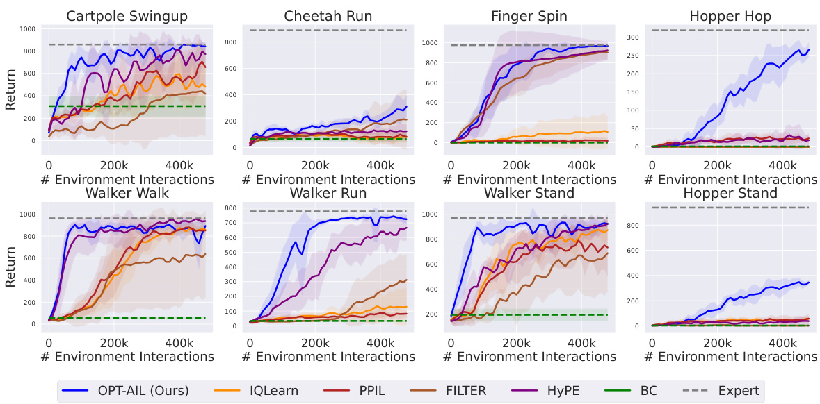
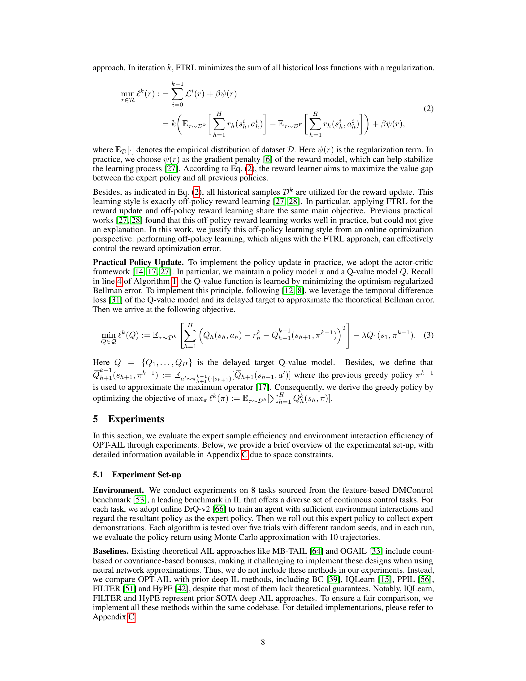
🔼 This figure compares the performance of OPT-AIL with several baselines across 8 different DMControl tasks. The performance is measured by the return, which represents the cumulative reward an agent receives during an episode. The x-axis shows the number of expert trajectories used for training, and the y-axis represents the average return achieved by each algorithm. Shaded regions indicate standard deviations over 5 independent runs, demonstrating the stability and consistency of the results. The figure highlights OPT-AIL’s superior performance across various tasks and its ability to achieve near-expert performance, even with limited expert data.

read the caption

Figure 1: Overall performance on 8 DMControl tasks over 5 random seeds following 500k interactions with the environment. Here the x-axis is the number of expert trajectories and the y-axis is the return. The solid lines are the mean of results while the shaded region corresponds to the standard deviation over 5 random seeds. Same as the following figures.

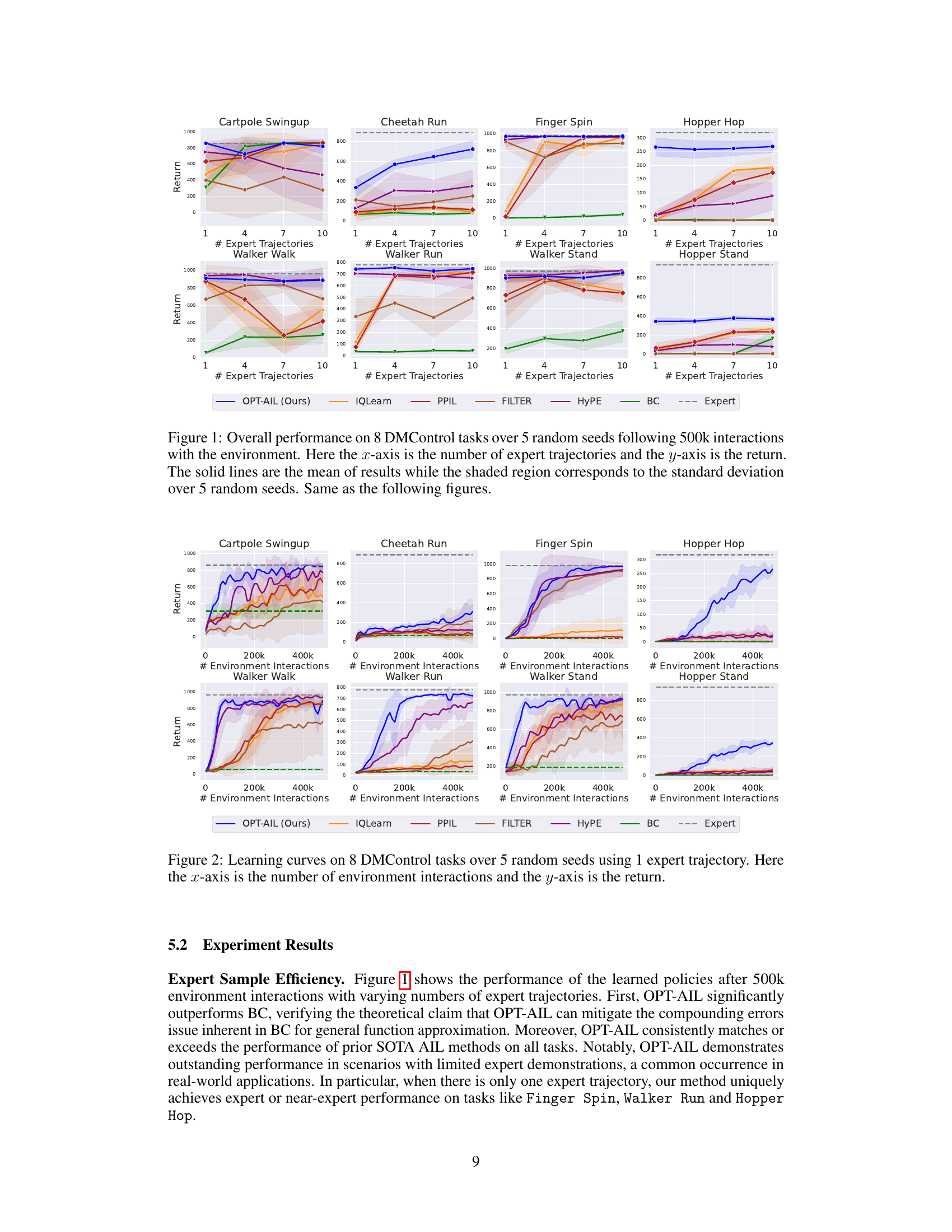
🔼 The figure displays the overall performance of OPT-AIL and other baseline algorithms across 8 different DMControl tasks. The x-axis represents the number of expert trajectories used for training, and the y-axis shows the average return achieved by each algorithm after 500,000 environment interactions. The solid lines represent the average return, and the shaded areas indicate the standard deviation over 5 different random seeds. The figure shows that OPT-AIL generally outperforms the baseline algorithms, especially when the number of expert trajectories is limited.

read the caption

Figure 1: Overall performance on 8 DMControl tasks over 5 random seeds following 500k interactions with the environment. Here the x-axis is the number of expert trajectories and the y-axis is the return. The solid lines are the mean of results while the shaded region corresponds to the standard deviation over 5 random seeds. Same as the following figures.

🔼 This figure presents the overall performance comparison of different imitation learning algorithms (OPT-AIL, IQLearn, PPIL, FILTER, HyPE, BC) against the expert policy on 8 diverse DMControl tasks. The performance is measured by the average return after 500,000 environment interactions. The x-axis represents the number of expert trajectories used for training, and the y-axis shows the average return achieved. Each line represents the average performance across five independent runs with different random seeds. The shaded area indicates the standard deviation.

read the caption

Figure 1: Overall performance on 8 DMControl tasks over 5 random seeds following 500k interactions with the environment. Here the x-axis is the number of expert trajectories and the y-axis is the return. The solid lines are the mean of results while the shaded region corresponds to the standard deviation over 5 random seeds. Same as the following figures.

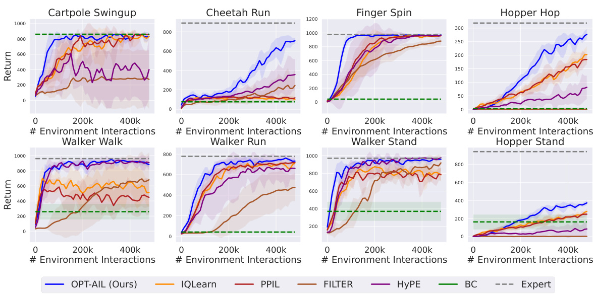
🔼 This figure presents the overall performance of OPT-AIL and other algorithms across 8 DMControl tasks using different numbers of expert trajectories. The x-axis represents the number of expert trajectories, while the y-axis shows the average return achieved by each algorithm after 500,000 interactions with the environment. The solid lines depict the average performance, while the shaded areas indicate the standard deviation across 5 different random seeds. The plot shows that OPT-AIL significantly outperforms other approaches, particularly when fewer expert trajectories are available.

read the caption

Figure 1: Overall performance on 8 DMControl tasks over 5 random seeds following 500k interactions with the environment. Here the x-axis is the number of expert trajectories and the y-axis is the return. The solid lines are the mean of results while the shaded region corresponds to the standard deviation over 5 random seeds. Same as the following figures.

Full paper

#