TL;DR#
Test-time training (TTT) allows neural networks to adapt to new data without retraining, but existing methods are often computationally expensive and require pre-training or augmentation. This paper addresses these limitations by proposing a novel architecture called Asynchronous Perception Machine (APM). Current TTT methods suffer from the information bottleneck problem, often relying on surrogate pre-text tasks, and using architectures like transformers that require parallel processing of all input patches. These limitations significantly increase computational costs and limit scalability.
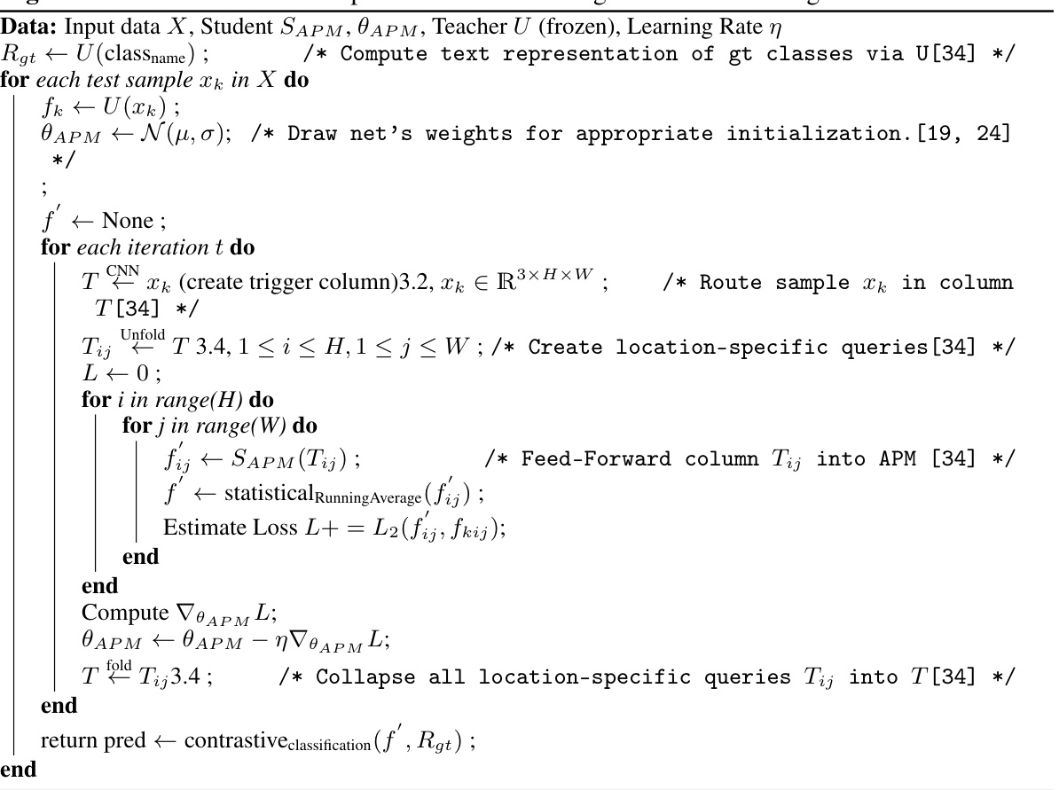
APM overcomes these challenges by processing image patches one at a time in any order, significantly reducing computational costs. It also learns directly from the test sample’s representation without any pre-training tasks or data augmentation, making it highly efficient and adaptable. The authors demonstrate APM’s competitive performance against existing TTT approaches, its scalability, and provide the first empirical evidence supporting the GLOM theory.
Key Takeaways#
Why does it matter?#
This paper is crucial for researchers in computer vision and machine learning because it introduces a novel test-time training architecture, APM, that significantly improves efficiency and performance. It offers a new perspective on machine perception, inspiring further research into efficient, scalable, and interpretable models. Its GLOM-inspired design opens new avenues for validating GLOM’s theoretical insights. The efficient nature of APM could lead to real-world applications requiring fast decision-making.
Visual Insights#

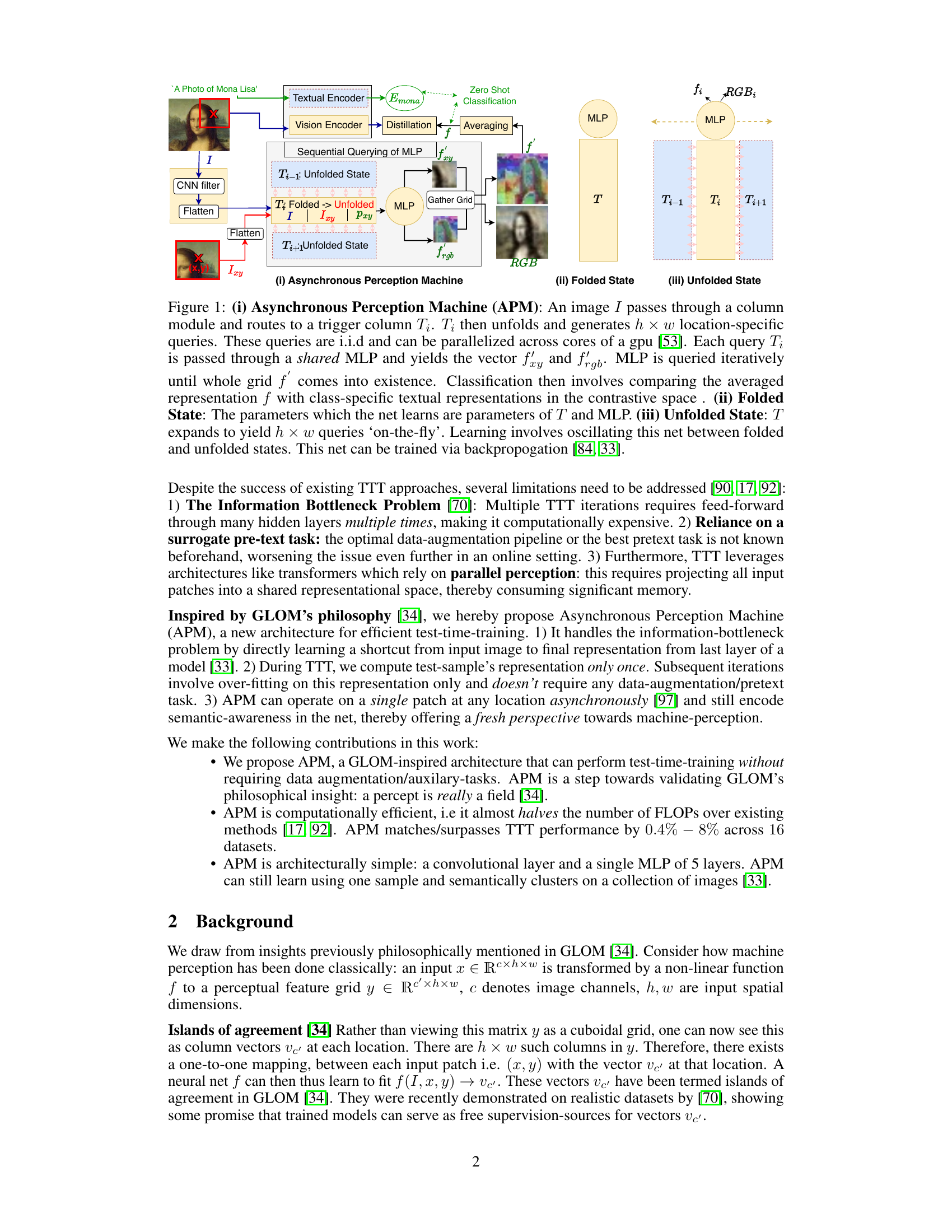
🔼 This figure illustrates the architecture of the Asynchronous Perception Machine (APM). Panel (i) shows the overall process, where an input image is processed sequentially through a column module and MLP to generate location-specific feature vectors. These vectors are then averaged and compared to textual representations for classification. Panel (ii) highlights the folded state of the network (parameters of T and MLP), while panel (iii) shows the unfolded state (h x w location-specific queries). The APM alternates between these folded and unfolded states during training and inference.
read the caption
Figure 1: (i) Asynchronous Perception Machine (APM): An image I passes through a column module and routes to a trigger column Ti. Ti then unfolds and generates h × w location-specific queries. These queries are i.i.d and can be parallelized across cores of a gpu [53]. Each query Ti is passed through a shared MLP and yields the vector fry and frgb. MLP is queried iteratively until whole grid f' comes into existence. Classification then involves comparing the averaged representation f with class-specific textual representations in the contrastive space. (ii) Folded State: The parameters which the net learns are parameters of T and MLP. (iii) Unfolded State: T expands to yield h × w queries ‘on-the-fly'. Learning involves oscillating this net between folded and unfolded states. This net can be trained via backpropogation [84, 33].

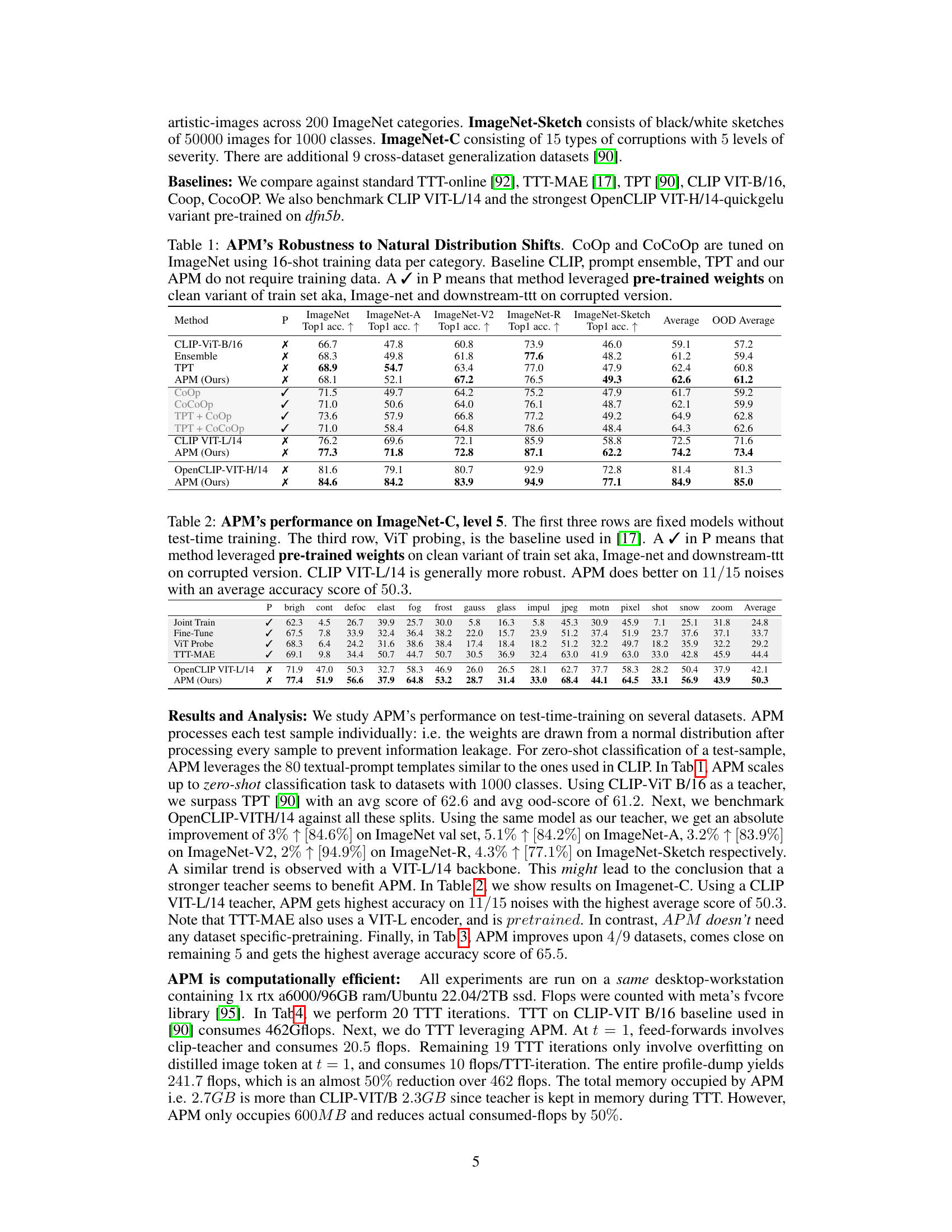
🔼 This table presents the robustness of different methods, including the proposed Asynchronous Perception Machine (APM), against natural distribution shifts. It compares the top-1 accuracy of various methods across several ImageNet datasets (ImageNet, ImageNet-A, ImageNet-V2, ImageNet-R, ImageNet-Sketch), which represent different types of distribution shifts (adversarial, corrupted, real-world, sketches). The table indicates whether each method used pre-trained weights and shows that APM performs competitively with or even better than other methods, even without pre-training or specific data augmentation techniques.
read the caption
Table 1: APM's Robustness to Natural Distribution Shifts. CoOp and CoCoOp are tuned on ImageNet using 16-shot training data per category. Baseline CLIP, prompt ensemble, TPT and our APM do not require training data. A ✓ in P means that method leveraged pre-trained weights on clean variant of train set aka, Image-net and downstream-ttt on corrupted version.
In-depth insights#
Async. Perception#
Asynchronous perception, a novel approach to machine perception, challenges conventional parallel processing by processing image patches asynchronously and independently. This method, unlike traditional parallel techniques, doesn’t require simultaneous processing of all input data. Instead, it prioritizes efficient processing by handling individual patches one at a time, in any order, significantly reducing computational burden. The system’s ability to encode semantic awareness despite its asynchronous nature is a key advantage. The use of a column module and a folding-unfolding mechanism is integral to the model’s unique architecture, facilitating efficient learning and feature extraction. The implications are vast, promising improvements in test-time training and potentially leading to innovative applications beyond the limitations of parallel processing paradigms. This approach aligns with the conceptual framework of GLOM, suggesting potential validation of its theory. Computational efficiency is a central benefit, drastically cutting down on the number of FLOPS needed for training and inference, thereby allowing for greater scalability and broader applicability.
GLOM-Inspired Arch.#
The heading ‘GLOM-Inspired Arch.’ suggests a significant departure from traditional neural network architectures. The core idea is likely to leverage the principles of the GLOM (Global-to-Local-Mapping) model, which proposes that perception is a field, not a sequence of discrete steps. This implies an architecture that processes information asynchronously and in parallel across locations, rather than sequentially layer by layer. A key characteristic is likely to be the absence of a fixed, predetermined processing order; instead, patches or regions of an input image may be processed in an arbitrary order, or even concurrently. This asynchronous processing is crucial for capturing the dynamic and parallel nature of perception in biological systems. Another key feature is likely to be a mechanism for efficient and incremental learning. This addresses the computational limitations of traditional test-time training methods which typically involve iterative feed-forward passes through many layers. The architecture will likely incorporate techniques for efficiently integrating new information without requiring full retraining, leading to a more adaptive and efficient model. Overall, a GLOM-inspired architecture promises a model with improved flexibility, computational efficiency, and biological plausibility in handling complex perception tasks.
TTT Efficiency#
The paper’s analysis of ‘TTT Efficiency’ centers on minimizing computational cost during test-time training. Asynchronous processing is key, enabling the model to handle image patches individually, significantly reducing FLOPs compared to traditional parallel methods. The core innovation lies in the Asynchronous Perception Machine (APM), an architecture designed to learn a compressed representation of the test sample efficiently in a single pass. This contrasts with existing TTT approaches that necessitate numerous forward passes across many layers. The effectiveness of this single-pass approach is further enhanced by a unique column folding-unfolding mechanism, allowing the model to efficiently process and learn from the sample’s information. The result is a substantial reduction in computational cost without sacrificing accuracy; APM almost halves FLOPs while maintaining competitive, and sometimes superior, performance. This efficiency makes APM particularly suitable for resource-constrained environments where real-time or low-latency decision-making is crucial. The paper’s experiments show that this efficiency gain is not at the cost of accuracy; in fact, it often surpasses other methods.
Island Emergence#
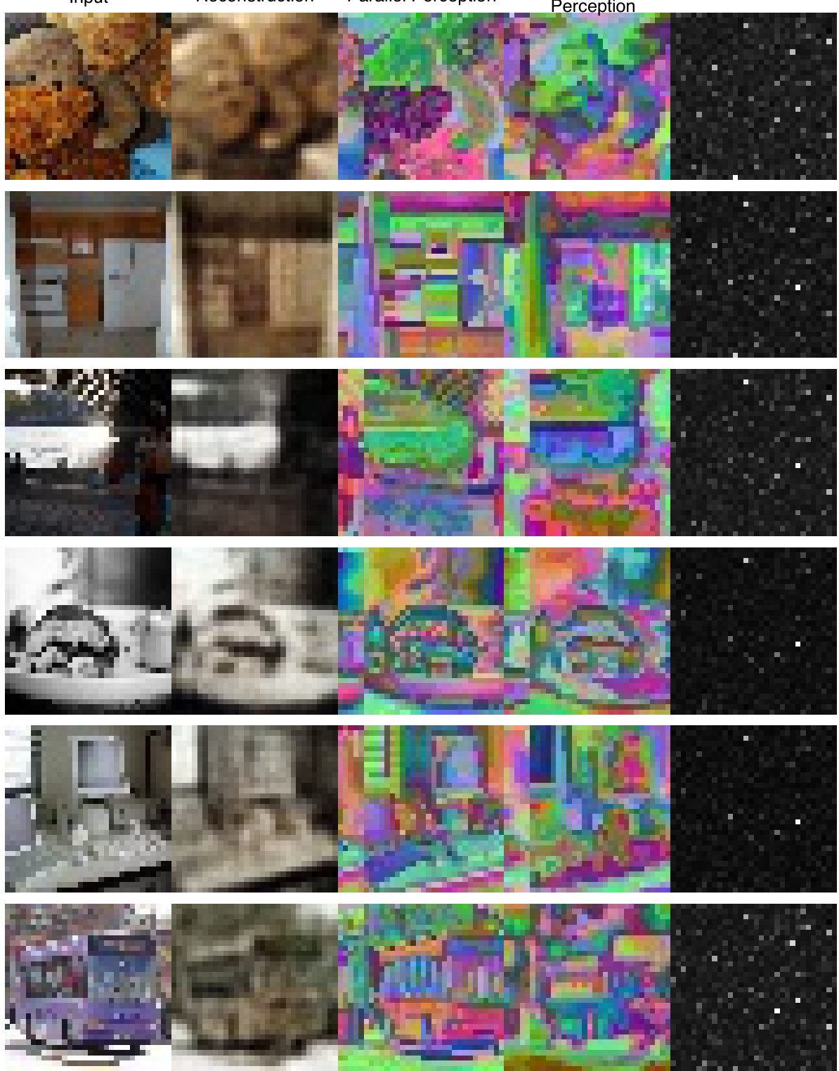
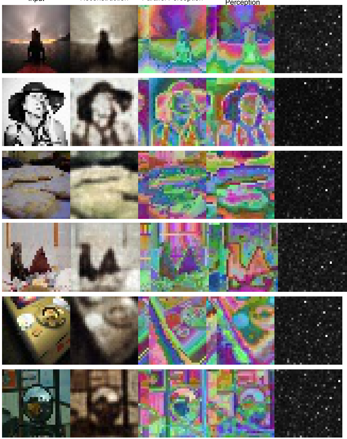
The concept of ‘Island Emergence’ in the context of neural networks, particularly within the framework of a GLOM-inspired architecture like APM, refers to the spontaneous formation of localized clusters of high-dimensional feature representations during test-time training. These ‘islands’ represent semantically coherent regions in the input data, emerging from the asynchronous processing of individual patches rather than through global, parallel computations. The emergence is a consequence of the network’s ability to iteratively refine its internal representation through test-time adaptation. The single-pass nature of feature extraction and subsequent overfitting allows the network to learn from just one sample and still capture the essence of the input, aligning with the principles of GLOM’s part-whole hierarchy. Crucially, this process is viewed as an implicit representation of the input scene, rather than explicit feature extraction. It validates GLOM’s theory of perception as a dynamic field, highlighting the computational efficiency and interpretability of APM’s approach. The ability to identify these islands without relying on dataset-specific pre-training, augmentation, or pretext tasks demonstrates a significant advance in zero-shot generalization and test-time adaptability.
Future Work#
The ‘Future Work’ section of a research paper on Asynchronous Perception Machines (APM) for efficient test-time training would naturally focus on extending the current capabilities and addressing limitations. Scaling APM to handle larger datasets and more complex tasks such as video understanding or 3D scene reconstruction is crucial. Investigating the impact of different architectural choices and hyperparameters on APM’s performance, particularly the number of MLP layers and the use of data augmentation, is vital. Exploring the theoretical underpinnings of APM’s ability to perform efficient test-time training and how it relates to the principles of GLOM (a related model) needs further investigation. Developing a deeper theoretical understanding of APM’s ability to perform one-sample overfitting is also paramount. This involves clarifying how and why this unique approach leads to improved test-time performance and generalization. Finally, the ‘Future Work’ should also discuss the implications of APM’s architecture for hardware implementation and deployment, exploring the potential of specialized hardware to fully leverage the efficiency gains offered by the asynchronous processing approach. Addressing ethical considerations and potential biases inherent in the model’s training and application would also round out the section.
More visual insights#
More on figures
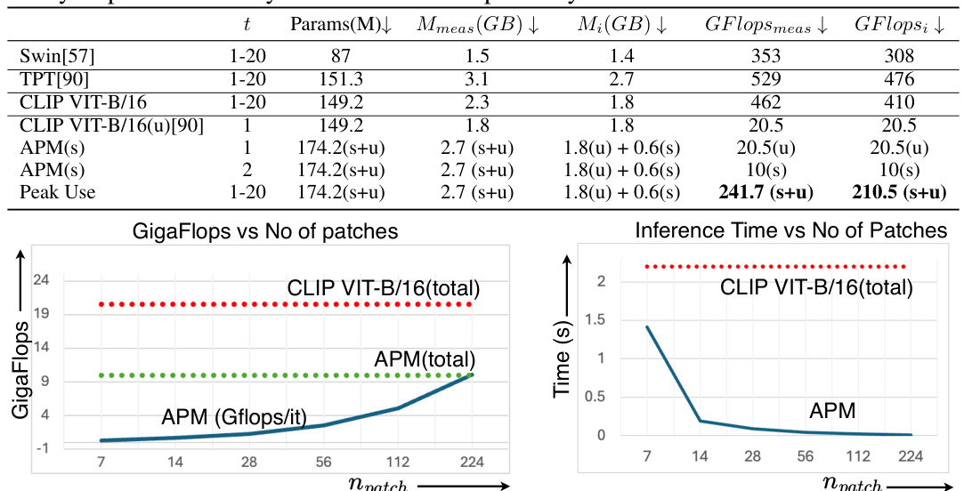
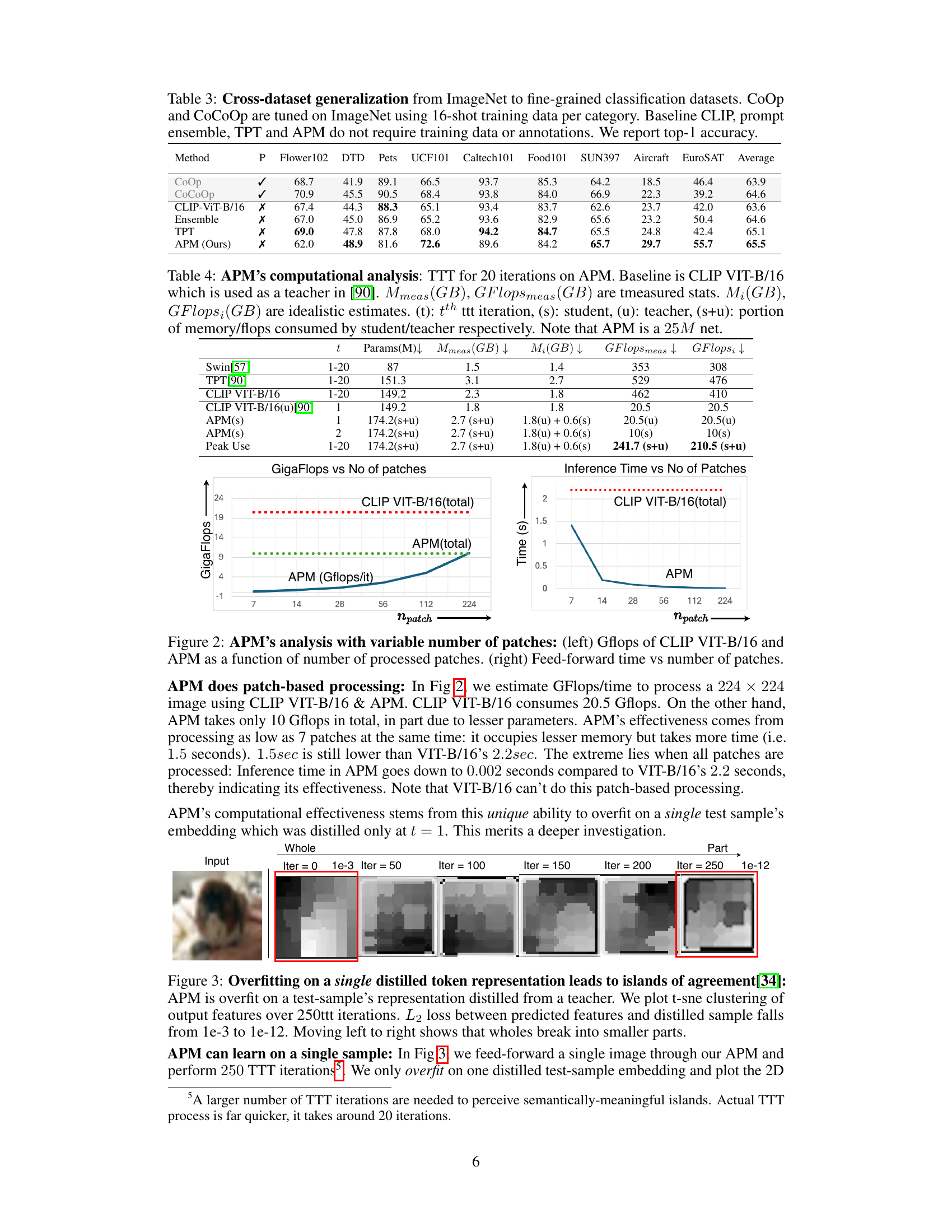
🔼 This figure demonstrates APM’s computational efficiency by comparing it against CLIP VIT-B/16 across varying numbers of image patches. The left panel shows the total number of GFLOPs (floating-point operations) required for processing, highlighting how APM’s patch-based processing significantly reduces computational cost compared to CLIP VIT-B/16’s parallel processing. The right panel illustrates the inference time for each method. Although APM might take slightly longer for a smaller number of patches, it significantly outperforms CLIP VIT-B/16 when processing many patches, emphasizing its scalability.
read the caption
Figure 2: APM's analysis with variable number of patches: (left) Gflops of CLIP VIT-B/16 and APM as a function of number of processed patches. (right) Feed-forward time vs number of patches.

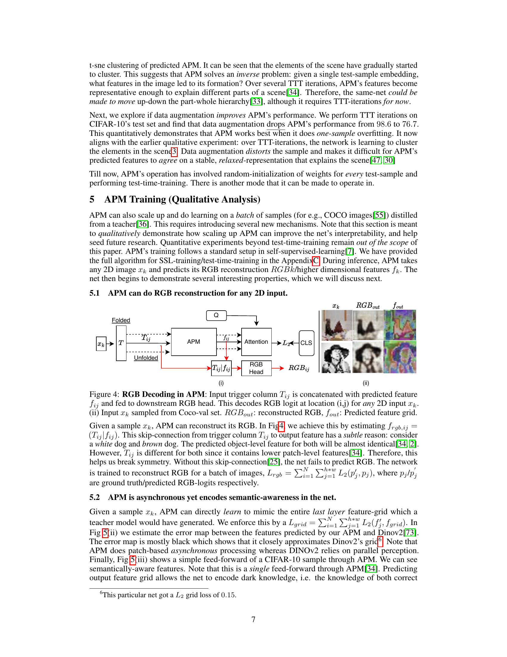
🔼 This figure visualizes the process of overfitting on a single distilled token representation using t-SNE clustering. It shows how, over 250 test-time training iterations, the initially holistic representation of the input image breaks down into smaller, more distinct parts, which are interpreted as islands of agreement. The L2 loss between the predicted and distilled features decreases significantly over these iterations, indicating successful overfitting.
read the caption
Figure 3: Overfitting on a single distilled token representation leads to islands of agreement[34]: APM is overfit on a test-sample's representation distilled from a teacher. We plot t-sne clustering of output features over 250ttt iterations. L2 loss between predicted features and distilled sample falls from le-3 to le-12. Moving left to right shows that wholes break into smaller parts.

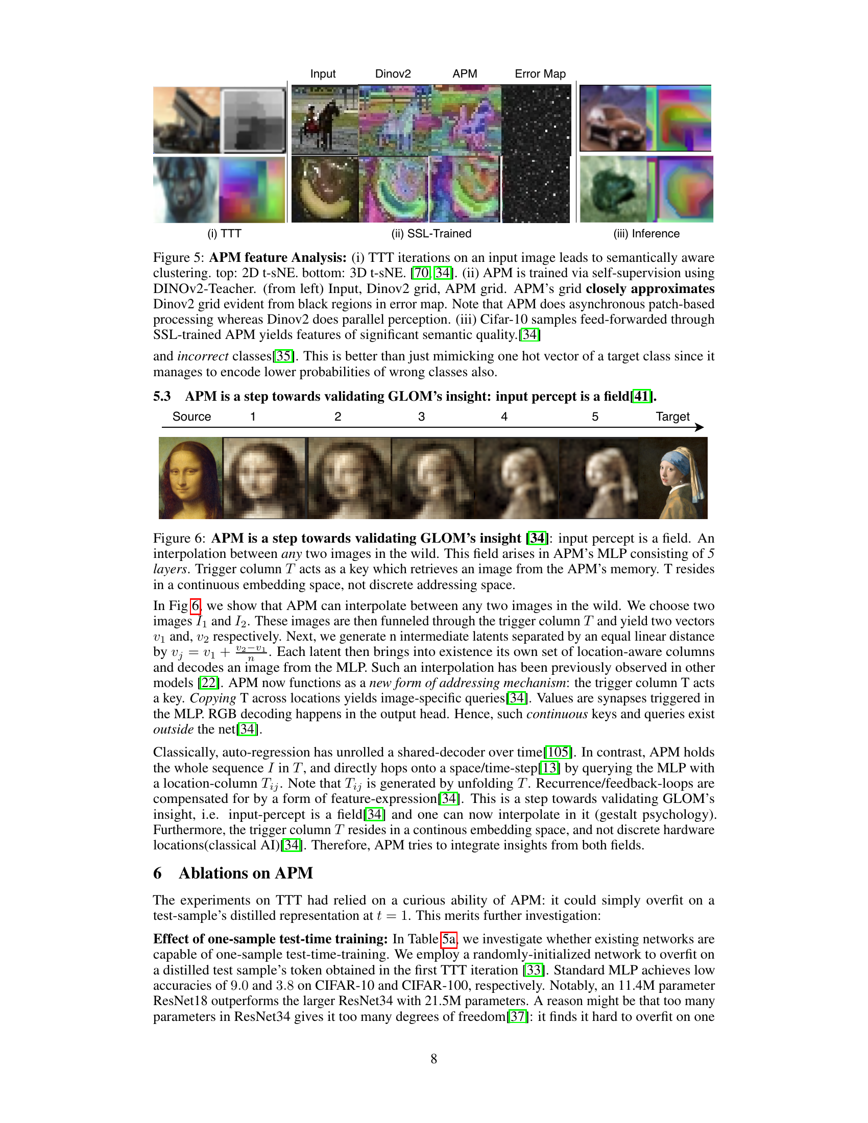
🔼 This figure illustrates how the Asynchronous Perception Machine (APM) reconstructs RGB values from an input image. It shows that the trigger column (Tij), containing an image’s identity, is combined with predicted features (fij) and fed to an RGB head to produce reconstructed RGB values (RGBout) and a feature grid (fout). The input image (xk) is from COCO-val dataset. This demonstrates APM’s ability to reconstruct RGB values directly from its internal representation, showcasing its efficiency and capacity for low-level perceptual tasks. The skip connection between the trigger column and the output layer helps break symmetry and improve RGB reconstruction.
read the caption
Figure 4: RGB Decoding in APM: Input trigger column Tij is concatenated with predicted feature fij and fed to downstream RGB head. This decodes RGB logit at location (i,j) for any 2D input Xk. (ii) Input xk sampled from Coco-val set. RGBout: reconstructed RGB, fout: Predicted feature grid.

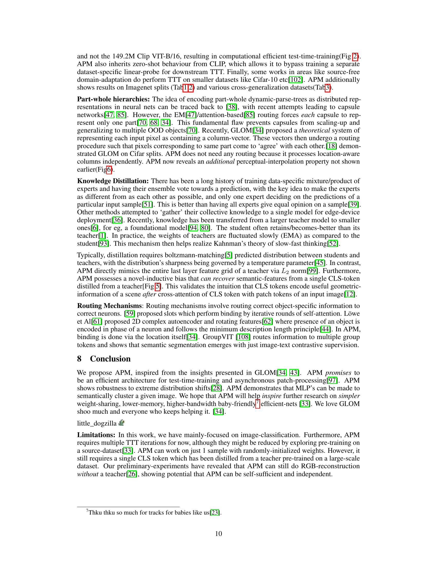
🔼 This figure shows the results of applying three different methods (TTT, SSL-trained, and inference) to image data using the Asynchronous Perception Machine (APM). The top row demonstrates that test-time training (TTT) with APM leads to semantically meaningful clustering of features in the image. The middle row compares the features extracted by APM to those extracted by DINOv2 after self-supervised training, showing a close approximation. The bottom row shows the semantically-aware features obtained through inference with a self-supervised trained APM.
read the caption
Figure 5: APM feature Analysis: (i) TTT iterations on an input image leads to semantically aware clustering. top: 2D t-sNE. bottom: 3D t-sNE. [70, 34]. (ii) APM is trained via self-supervision using DINOv2-Teacher. (from left) Input, Dinov2 grid, APM grid. APM's grid closely approximates Dinov2 grid evident from black regions in error map. Note that APM does asynchronous patch-based processing whereas Dinov2 does parallel perception. (iii) Cifar-10 samples feed-forwarded through SSL-trained APM yields features of significant semantic quality.[34]

🔼 This figure demonstrates the ability of APM to interpolate between two images. The trigger column, T, acts as a key to retrieve images from APM’s internal representation, a continuous embedding space rather than discrete addressing. This interpolation highlights the concept of the input percept as a field, a core tenet of GLOM.
read the caption
Figure 6: APM is a step towards validating GLOM's insight [34]: input percept is a field. An interpolation between any two images in the wild. This field arises in APM's MLP consisting of 5 layers. Trigger column T acts as a key which retrieves an image from the APM's memory. T resides in a continuous embedding space, not discrete addressing space.
🔼 This figure illustrates the architecture of the Asynchronous Perception Machine (APM). Panel (i) shows the overall process: an image is processed sequentially by a column module, which generates location-specific queries. These queries are processed through a shared MLP, resulting in a feature grid. Finally, a classifier compares the averaged feature representation with textual representations for classification. Panel (ii) depicts the ‘folded’ state of the network, showing only the learned parameters (T and MLP weights). Panel (iii) shows the ‘unfolded’ state, illustrating the generation of multiple queries from a single column during operation. The network’s training involves switching between these folded and unfolded states using backpropagation.
read the caption
Figure 1: (i) Asynchronous Perception Machine (APM): An image I passes through a column module and routes to a trigger column Ti. Ti then unfolds and generates h × w location-specific queries. These queries are i.i.d and can be parallelized across cores of a gpu [53]. Each query Ti is passed through a shared MLP and yields the vector fxy and frgb. MLP is queried iteratively until whole grid f' comes into existence. Classification then involves comparing the averaged representation f with class-specific textual representations in the contrastive space. (ii) Folded State: The parameters which the net learns are parameters of T and MLP. (iii) Unfolded State: T expands to yield h × w queries ‘on-the-fly’. Learning involves oscillating this net between folded and unfolded states. This net can be trained via backpropogation [84, 33].

🔼 This figure visualizes the results of applying the proposed Asynchronous Perception Machine (APM) model on CIFAR-10 dataset. The image shows a collection of 20 image patches extracted from the dataset, with each patch accompanied by the corresponding feature map generated by APM. The visualization technique used is t-SNE, which projects the high-dimensional feature maps into a 2D space for visualization. The resulting visualization reveals distinct clusters of features corresponding to different parts and wholes of objects present in the image patches. The caption highlights that these clusters or ‘islands’ emerge organically without any manual selection or pre-processing of the data, demonstrating the model’s ability to capture meaningful, semantically-aware feature representations.
read the caption
Figure 7: Cifar 10 islands: Individual part-wholes are clearly observed in APM features. These features are used for downstream classification. We leverage the visualization mechanism by [70]. These islands are not been hand-picked.[34]

🔼 This figure shows the architecture of Asynchronous Perception Machine (APM). It is composed of three parts: (i) APM architecture, which shows how an image is processed asynchronously through a column module and MLPs to generate location-specific queries; (ii) Folded state, showing that the learnable parameters are those of the trigger column and MLP; and (iii) Unfolded state, illustrating the expansion of the trigger column into multiple location-aware queries. The process involves oscillating between folded and unfolded states for training using backpropagation.
read the caption
Figure 1: (i) Asynchronous Perception Machine (APM): An image I passes through a column module and routes to a trigger column Ti. Ti then unfolds and generates h × w location-specific queries. These queries are i.i.d and can be parallelized across cores of a gpu [53]. Each query Ti is passed through a shared MLP and yields the vector fxy and frgb. MLP is queried iteratively until whole grid f’ comes into existence. Classification then involves comparing the averaged representation f with class-specific textual representations in the contrastive space. (ii) Folded State: The parameters which the net learns are parameters of T and MLP. (iii) Unfolded State: T expands to yield h × w queries ‘on-the-fly’. Learning involves oscillating this net between folded and unfolded states. This net can be trained via backpropogation [84, 33].

🔼 This figure shows the architecture of the Asynchronous Perception Machine (APM). Panel (i) illustrates the overall process, where an image is processed asynchronously patch by patch via a column module and MLP. Panel (ii) shows the ‘folded state’ of the network (its learnable parameters), while panel (iii) displays the ‘unfolded state’ representing the expanded set of queries processed during training.
read the caption
Figure 1: (i) Asynchronous Perception Machine (APM): An image I passes through a column module and routes to a trigger column Ti. Ti then unfolds and generates h × w location-specific queries. These queries are i.i.d and can be parallelized across cores of a gpu [53]. Each query Ti is passed through a shared MLP and yields the vector fxy and frgb. MLP is queried iteratively until whole grid f' comes into existence. Classification then involves comparing the averaged representation f with class-specific textual representations in the contrastive space. (ii) Folded State: The parameters which the net learns are parameters of T and MLP. (iii) Unfolded State: T expands to yield h × w queries ‘on-the-fly’. Learning involves oscillating this net between folded and unfolded states. This net can be trained via backpropogation [84, 33].
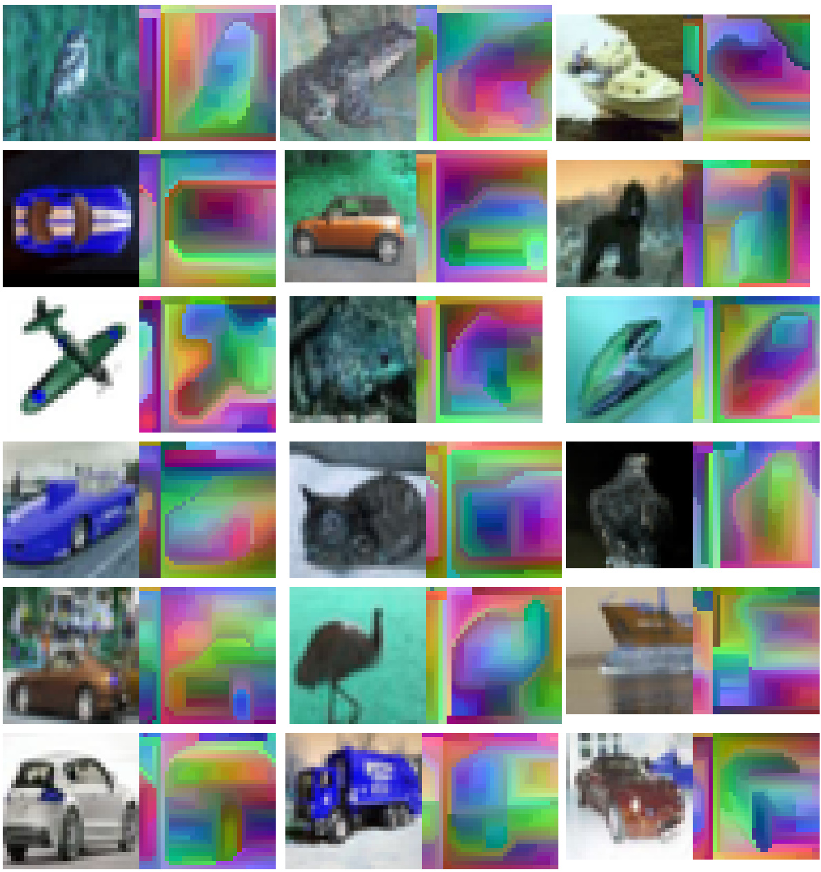
🔼 This figure visualizes features extracted from the APM model trained on CIFAR-10. Each image shows an input image alongside its corresponding feature representation generated by the APM. The feature maps are visualized using a t-SNE dimensionality reduction technique, which reveals distinct clusters (islands) of features corresponding to different parts of the objects in the input images. The visualization highlights the model’s ability to capture semantically meaningful features by clustering related parts of objects together, demonstrating the model’s capacity for part-whole representation learning. Importantly, these clusters were not manually selected, indicating that APM’s feature representation naturally forms these semantically relevant groupings.
read the caption
Figure 7: Cifar 10 islands: Individual part-wholes are clearly observed in APM features. These features are used for downstream classification. We leverage the visualization mechanism by [70]. These islands are not been hand-picked[34]
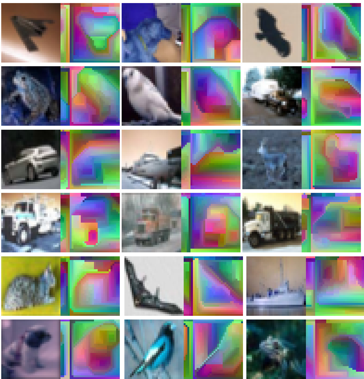
🔼 This figure visualizes the features learned by the Asynchronous Perception Machine (APM) on the CIFAR-10 dataset. Each image shows a different object from CIFAR-10, with its corresponding feature representation generated by APM. The color patterns within the feature representations highlight distinct parts and sub-parts within the objects, demonstrating the model’s ability to learn and represent part-whole relationships. The caption emphasizes that these representations, referred to as ‘islands’, are not hand-picked but emerge naturally from the model’s learning process. This visualization uses a technique from [70] to project the high-dimensional features into a 2D space while preserving spatial relationships.
read the caption
Figure 7: Cifar 10 islands: Individual part-wholes are clearly observed in APM features. These features are used for downstream classification. We leverage the visualization mechanism by [70]. These islands are not been hand-picked.[34]

🔼 This figure illustrates the architecture of the Asynchronous Perception Machine (APM), showing how it processes an image asynchronously, patch by patch, using a column module and MLPs. It highlights the folded and unfolded states of the network, crucial to the training process, and the final classification stage which compares averaged representations to textual representations.
read the caption
Figure 1: (i) Asynchronous Perception Machine (APM): An image I passes through a column module and routes to a trigger column Ti. Ti then unfolds and generates h × w location-specific queries. These queries are i.i.d and can be parallelized across cores of a gpu [53]. Each query Ti is passed through a shared MLP and yields the vector fxy and frgb. MLP is queried iteratively until whole grid f' comes into existence. Classification then involves comparing the averaged representation f with class-specific textual representations in the contrastive space. (ii) Folded State: The parameters which the net learns are parameters of T and MLP. (iii) Unfolded State: T expands to yield h × w queries ‘on-the-fly’. Learning involves oscillating this net between folded and unfolded states. This net can be trained via backpropogation [84, 33].
🔼 This figure shows the architecture of the Asynchronous Perception Machine (APM). It illustrates how an image is processed asynchronously, one patch at a time, using a column module and MLPs. The figure highlights the folded and unfolded states of the network during the training process. It also visually represents the process of querying the MLP iteratively to generate a complete feature grid. Finally, it shows how classification is performed by comparing the averaged representation to textual representations.
read the caption
Figure 1: (i) Asynchronous Perception Machine (APM): An image I passes through a column module and routes to a trigger column Ti. Ti then unfolds and generates h × w location-specific queries. These queries are i.i.d and can be parallelized across cores of a gpu [53]. Each query Ti is passed through a shared MLP and yields the vector fxy and frgb. MLP is queried iteratively until whole grid f' comes into existence. Classification then involves comparing the averaged representation f with class-specific textual representations in the contrastive space. (ii) Folded State: The parameters which the net learns are parameters of T and MLP. (iii) Unfolded State: T expands to yield h × w queries ‘on-the-fly’. Learning involves oscillating this net between folded and unfolded states. This net can be trained via backpropogation [84, 33].
🔼 This figure illustrates the architecture of the Asynchronous Perception Machine (APM). Panel (i) shows the overall process flow, highlighting the sequential querying of MLPs to process image patches asynchronously. The system alternates between a ‘folded’ state (ii), where parameters are learned, and an ‘unfolded’ state (iii), where h x w location-specific queries are generated on-the-fly. This dynamic unfolding and folding process allows for efficient test-time training.
read the caption
Figure 1: (i) Asynchronous Perception Machine (APM): An image I passes through a column module and routes to a trigger column Ti. Ti then unfolds and generates h × w location-specific queries. These queries are i.i.d and can be parallelized across cores of a gpu [53]. Each query Ti is passed through a shared MLP and yields the vector fxy and frgb. MLP is queried iteratively until whole grid f' comes into existence. Classification then involves comparing the averaged representation f with class-specific textual representations in the contrastive space. (ii) Folded State: The parameters which the net learns are parameters of T and MLP. (iii) Unfolded State: T expands to yield h × w queries ‘on-the-fly'. Learning involves oscillating this net between folded and unfolded states. This net can be trained via backpropogation [84, 33].
More on tables

🔼 This table presents the performance of APM and several baseline models on ImageNet-C, a dataset with 15 types of image corruptions at 5 severity levels. The baseline models are not using test time training. It shows the robustness of the different methods to the image corruptions. APM’s performance is compared to others both with and without pre-trained weights.
read the caption
Table 2: APM's performance on ImageNet-C, level 5. The first three rows are fixed models without test-time training. The third row, ViT probing, is the baseline used in [17]. A ✓ in P means that method leveraged pre-trained weights on clean variant of train set aka, Image-net and downstream-ttt on corrupted version.

🔼 This table presents a comparison of the performance of various methods, including the proposed Asynchronous Perception Machine (APM), on ImageNet and several out-of-distribution (OOD) datasets. It highlights APM’s ability to achieve competitive performance without requiring dataset-specific pre-training or augmentation. The ‘P’ column indicates whether a method used pre-trained weights on a clean ImageNet dataset before being tested on the OOD datasets. The table showcases APM’s robustness to various types of image corruptions and distribution shifts.
read the caption
Table 1: APM's Robustness to Natural Distribution Shifts. CoOp and CoCoOp are tuned on ImageNet using 16-shot training data per category. Baseline CLIP, prompt ensemble, TPT and our APM do not require training data. A ✓ in P means that method leveraged pre-trained weights on clean variant of train set aka, Image-net and downstream-ttt on corrupted version.

🔼 This ablation study investigates the impact of different design choices on APM’s performance. It compares the accuracy of various models (including baselines like CLIP ViT-L/14, MLP, ResNet18, and ResNet34) on CIFAR-10 and CIFAR-100 datasets using different combinations of loss functions (Lgrid, Lcls, Lrgb) and trigger column configurations (Tc, Tvit). The results demonstrate the effectiveness of the proposed APM architecture and specific design choices in achieving high accuracy.
read the caption
Table 5: Ablations on APM. All nets except CLIP VIT-L/14 use random weights b) Tc: trigger column contains convolutions. Tvit: Trigger column contains a routed VIT representation. C-10: CIFAR-10, C-100: CIFAR-100. Accuracy is reported.

🔼 This table compares the performance of APM against several other methods on various image classification datasets with natural distribution shifts. The datasets include ImageNet, ImageNet-A, ImageNet-V2, ImageNet-R, and ImageNet-Sketch. The table highlights APM’s robustness by showing competitive results even without dataset-specific pre-training, augmentation or any pretext task, unlike methods that leverage pre-trained weights.
read the caption
Table 1: APM's Robustness to Natural Distribution Shifts. CoOp and CoCoOp are tuned on ImageNet using 16-shot training data per category. Baseline CLIP, prompt ensemble, TPT and our APM do not require training data. A ✓ in P means that method leveraged pre-trained weights on clean variant of train set aka, Image-net and downstream-ttt on corrupted version.

🔼 This table presents a comparison of the performance of various methods on different ImageNet datasets with varying levels of corruption or distribution shifts. It highlights APM’s robustness to these shifts, even without dataset-specific pre-training, augmentation, or pretext tasks, and its competitive performance against existing state-of-the-art methods. The ‘P’ column indicates whether pre-trained weights were used.
read the caption
Table 1: APM's Robustness to Natural Distribution Shifts. CoOp and CoCoOp are tuned on ImageNet using 16-shot training data per category. Baseline CLIP, prompt ensemble, TPT and our APM do not require training data. A ✓ in P means that method leveraged pre-trained weights on clean variant of train set aka, Image-net and downstream-ttt on corrupted version.

🔼 This table presents the performance comparison of different methods on various image classification tasks with natural distribution shifts. It includes baseline methods such as CLIP, prompt ensemble, and TPT, along with methods that leverage pre-trained weights. The table shows the top-1 accuracy for each method on ImageNet, ImageNet-A, ImageNet-V2, ImageNet-R, and ImageNet-Sketch. The results demonstrate APM’s robustness in handling distribution shifts, showing competitive performance to the state-of-the-art methods, while not requiring additional training data.
read the caption
Table 1: APM's Robustness to Natural Distribution Shifts. CoOp and CoCoOp are tuned on ImageNet using 16-shot training data per category. Baseline CLIP, prompt ensemble, TPT and our APM do not require training data. A ✓ in P means that method leveraged pre-trained weights on clean variant of train set aka, Image-net and downstream-ttt on corrupted version.

🔼 This table presents a comparison of different models’ performance on ImageNet-C, a dataset with 15 types of image corruptions at level 5 severity. The models include fixed models without test-time training (TTT), a ViT probing baseline, and the proposed APM model. The table shows the accuracy achieved by each model for various noise types, highlighting APM’s superior performance on 11 out of 15 noise types, with an overall average accuracy of 50.3%. The ‘P’ column indicates whether pre-trained weights were used.
read the caption
Table 2: APM's performance on ImageNet-C, level 5. The first three rows are fixed models without test-time training. The third row, ViT probing, is the baseline used in [17]. A ✓ in P means that method leveraged pre-trained weights on clean variant of train set aka, Image-net and downstream-ttt on corrupted version. CLIP VIT-L/14 is generally more robust. APM does better on 11/15 noises with an average accuracy score of 50.3.

🔼 This table shows the results of an ablation study on the APM model, specifically focusing on the impact of varying the number of parameters in its linear layers. The experiment was conducted on the DTD dataset, and the results show that increasing the number of parameters from 7M to 53M leads to a gradual improvement in the top-1 classification accuracy, reaching a peak of 49.1%. However, further increases in the number of parameters beyond 53M result in a decrease in accuracy, indicating that the model starts to overfit. The table provides a quantitative analysis of the optimal parameter count for APM on the DTD dataset.
read the caption
Table 9: Ablation on APM parameter count on DTD dataset: Increasing the number of parameters to 53M improves APM's performance to 49.1 beyond which it starts to drop. Top 1 classification accuracy is being reported.

🔼 This table presents a comparison of the performance of various methods, including APM, on ImageNet-C, which is a dataset with 15 types of image corruptions at level 5 severity. The first three rows show results from models without test-time training. The table highlights APM’s superior performance compared to other methods, especially on a majority of the noise types, with an overall average accuracy of 50.3%.
read the caption
Table 2: APM's performance on ImageNet-C, level 5. The first three rows are fixed models without test-time training. The third row, ViT probing, is the baseline used in [17]. A ✓ in P means that method leveraged pre-trained weights on clean variant of train set aka, Image-net and downstream-ttt on corrupted version. CLIP VIT-L/14 is generally more robust. APM does better on 11/15 noises with an average accuracy score of 50.3.

🔼 This table presents the performance comparison of APM against other methods on ImageNet-C dataset with corruption level 5. It shows the accuracy of each method for each type of noise. The table highlights APM’s superior performance on 11 out of 15 noise types, demonstrating its robustness and achieving an average accuracy score of 50.3%.
read the caption
Table 2: APM's performance on ImageNet-C, level 5. The first three rows are fixed models without test-time training. The third row, ViT probing, is the baseline used in [17]. A ✓ in P means that method leveraged pre-trained weights on clean variant of train set aka, Image-net and downstream-ttt on corrupted version. CLIP VIT-L/14 is generally more robust. APM does better on 11/15 noises with an average accuracy score of 50.3.

🔼 This table presents a comparison of the performance of different models on ImageNet-C, specifically at level 5 corruption. It shows the accuracy of several models (including the proposed APM) on various types of image noise. The baseline model uses pre-trained weights. The results demonstrate APM’s ability to outperform existing methods on a majority of noise types.
read the caption
Table 2: APM's performance on ImageNet-C, level 5. The first three rows are fixed models without test-time training. The third row, ViT probing, is the baseline used in [17]. A ✓ in P means that method leveraged pre-trained weights on clean variant of train set aka, Image-net and downstream-ttt on corrupted version. CLIP VIT-L/14 is generally more robust. APM does better on 11/15 noises with an average accuracy score of 50.3.

🔼 This table compares the performance of APM against other methods on ImageNet-C, level 5, a dataset with 15 types of image corruptions. The results show the top-1 accuracy for each corruption type. It highlights that while some methods use pre-trained weights, APM does not, yet still achieves competitive or superior performance. The average accuracy across all corruptions demonstrates APM’s robustness.
read the caption
Table 2: APM's performance on ImageNet-C, level 5. The first three rows are fixed models without test-time training. The third row, ViT probing, is the baseline used in [17]. A ✓ in P means that method leveraged pre-trained weights on clean variant of train set aka, Image-net and downstream-ttt on corrupted version. CLIP VIT-L/14 is generally more robust. APM does better on 11/15 noises with an average accuracy score of 50.3.

🔼 This table compares the performance of APM against other methods on ImageNet-C, level 5, a dataset with 15 types of image corruptions. It shows that APM outperforms several baselines on 11 out of 15 noise types. The table highlights APM’s robustness to image corruptions without relying on pre-trained weights or data augmentation.
read the caption
Table 2: APM's performance on ImageNet-C, level 5. The first three rows are fixed models without test-time training. The third row, ViT probing, is the baseline used in [17]. A ✓ in P means that method leveraged pre-trained weights on clean variant of train set aka, Image-net and downstream-ttt on corrupted version. CLIP VIT-L/14 is generally more robust. APM does better on 11/15 noises with an average accuracy score of 50.3.
Full paper#
