TL;DR#
Inverse Reinforcement Learning (IRL) aims to infer an agent’s reward function by observing its behavior, assuming the agent acts optimally. However, IRL often suffers from ambiguity, as many reward functions can explain the same behavior. Moreover, real-world scenarios rarely provide only optimal demonstrations; often, sub-optimal demonstrations are also available. This is particularly challenging when dealing with human-in-the-loop scenarios where obtaining truly optimal demonstrations may be difficult or costly. This paper addresses this crucial limitation.
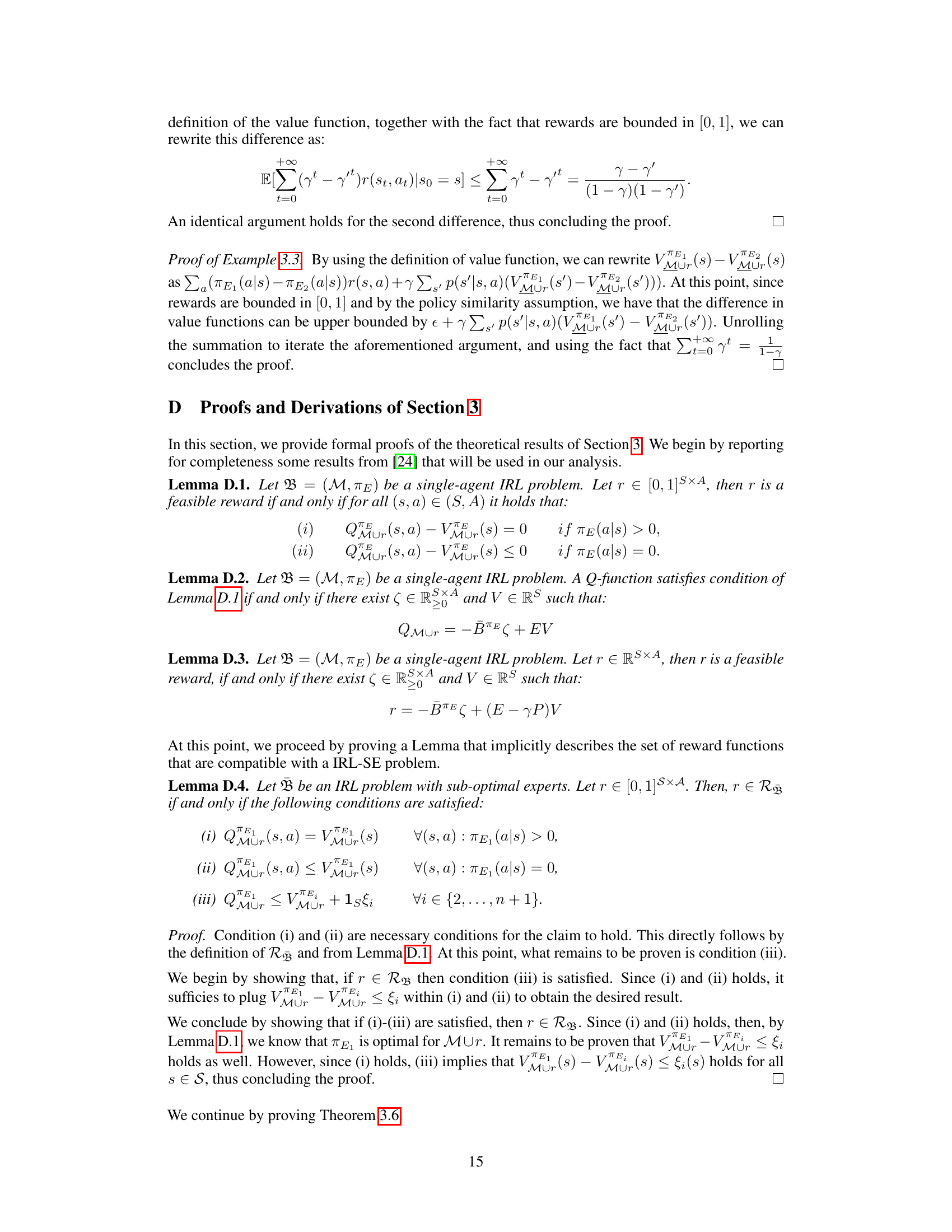
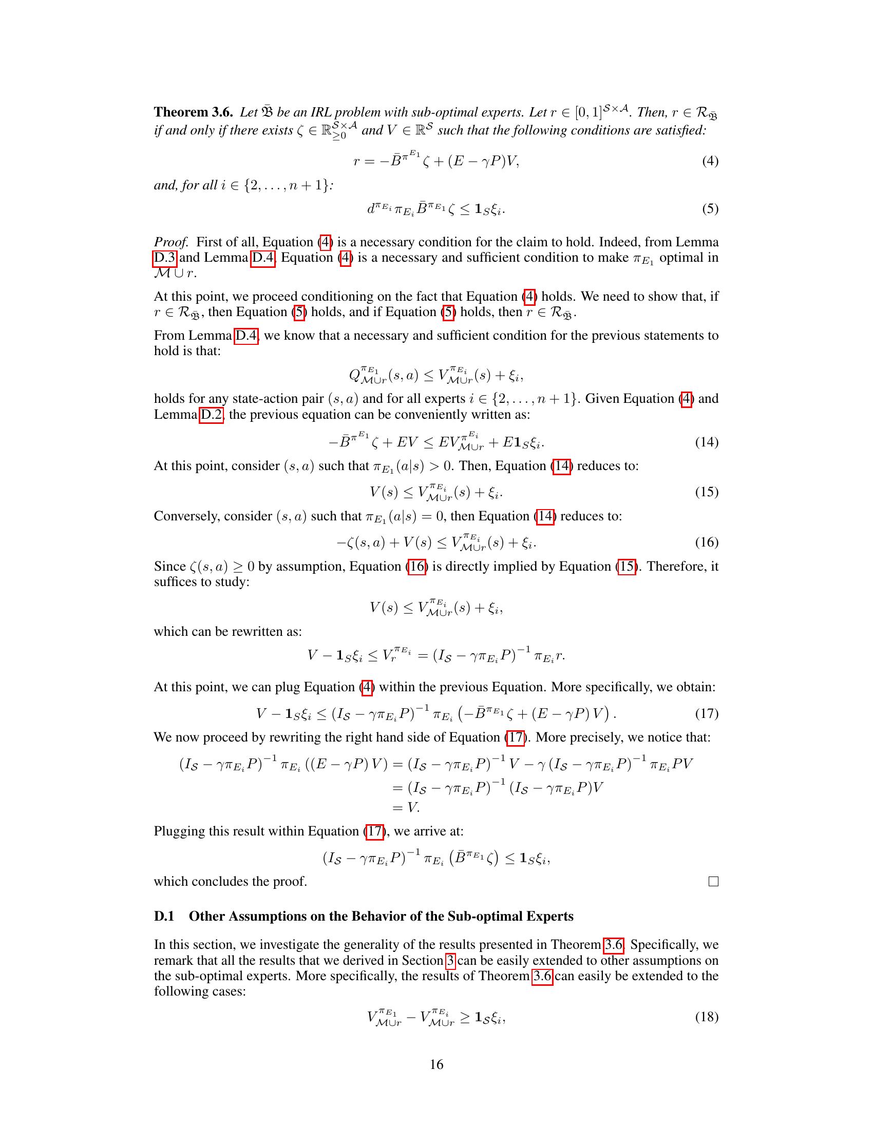
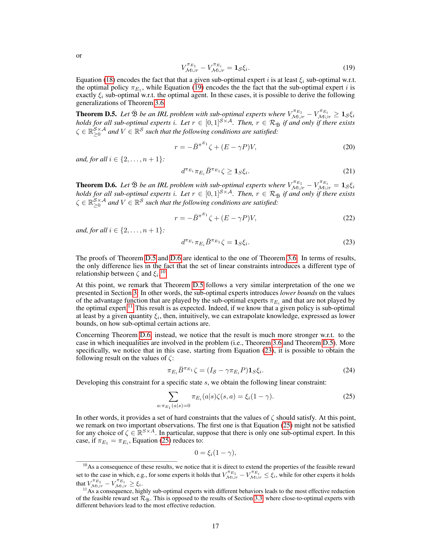
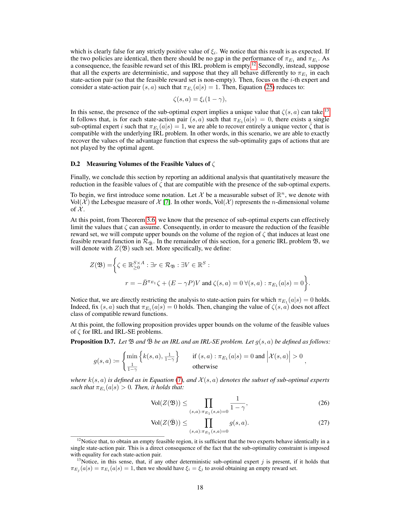
This research proposes a novel approach to IRL that leverages data from multiple experts, including sub-optimal ones. The study shows that including sub-optimal expert data significantly reduces the ambiguity of the reward estimation in IRL. The authors present a theoretical analysis of the problem with sub-optimal experts, showing that this approach effectively shrinks the set of plausible reward functions. Further, they propose a uniform sampling algorithm and prove its optimality under certain conditions. This work offers valuable theoretical insights and practical solutions to a critical issue in IRL.
Key Takeaways#
Why does it matter?#
This paper is crucial because it tackles a significant challenge in Inverse Reinforcement Learning (IRL): ambiguity. By introducing sub-optimal expert demonstrations, it offers a novel approach to reduce uncertainty in reward function estimation. This opens new avenues for applications where perfect expert data is scarce, improving the robustness and reliability of IRL algorithms. The rigorous theoretical analysis further enhances the paper’s value, providing strong foundations for future research in this area.
Visual Insights#

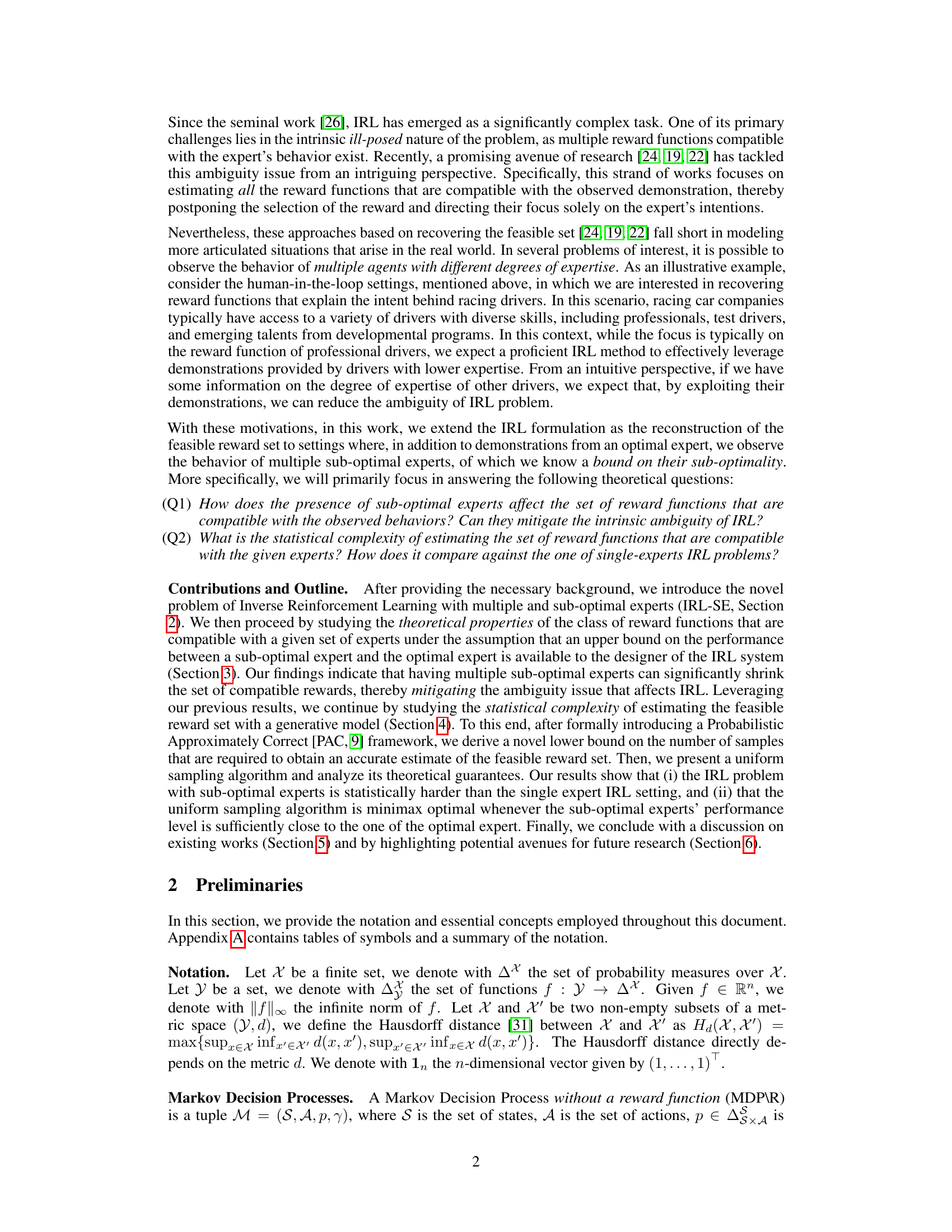
🔼 This figure shows a simple Markov Decision Process (MDP) with two states (S₀ and S₁) and two actions (A₁ and A₂). The optimal expert (πΕ₁) always chooses action A₁ when in state S₀ and transitions to state S₁. The sub-optimal expert (πΕᵢ) also chooses action A₁ from S₀ (it is sub-optimal in S₀). Both experts act identically in state S₁: they choose action A. This example demonstrates that even if sub-optimal agents behave similarly to optimal agents in certain states, their inclusion can impact the feasible set of rewards. The differences in behavior between the optimal and sub-optimal agents in S₀ allows the sub-optimal experts to reduce ambiguity in the inverse reinforcement learning (IRL) problem, as noted in Example 3.5 of the paper.
read the caption
Figure 1: MDP example, with 2 states and 2 experts, that highlights the benefits of sub-optimal experts (Example 3.5). In S₁ both ΠΕ₁ and ΠΕ; are identical, i.e., πε₁ (Ā|S1) = πε₁ (A|S1) = 1.

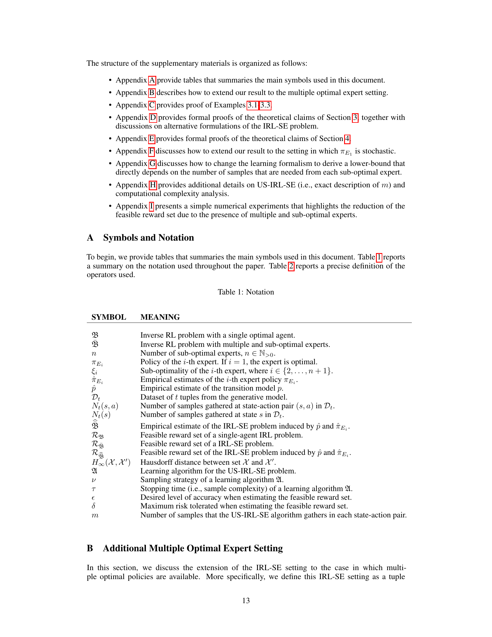
🔼 This table summarizes the notations used in the paper. It lists symbols and their meanings, including those related to the Inverse Reinforcement Learning (IRL) problem with a single optimal expert, the IRL problem with multiple sub-optimal experts, the number of sub-optimal experts, policies of experts, sub-optimality of experts, empirical estimates, datasets, and feasible reward sets for both single and multiple expert settings. It also defines the Hausdorff distance, the learning algorithm, sampling strategy, sample complexity, accuracy, and risk parameters.
read the caption
Table 1: Notation
In-depth insights#
Suboptimal IRL#
Suboptimal Inverse Reinforcement Learning (IRL) tackles the inherent ambiguity of standard IRL by leveraging demonstrations from agents exhibiting varying degrees of optimality. Instead of relying solely on a perfect expert, suboptimal IRL incorporates data from less-skilled agents, enriching the learning process and potentially mitigating the ill-posed nature of reward function recovery. This approach acknowledges the reality of real-world scenarios where obtaining perfect demonstrations is often impractical. By analyzing the discrepancies between optimal and suboptimal behaviors, suboptimal IRL can constrain the space of plausible reward functions, refining the estimate and enhancing the robustness of the learned model. The theoretical implications are significant, as suboptimal IRL addresses the issue of identifiability in standard IRL, providing a more reliable and practical framework for various applications.
Feasible Reward Set#
The concept of a ‘feasible reward set’ is central to addressing the inherent ambiguity in Inverse Reinforcement Learning (IRL). In standard IRL, observing an expert’s behavior doesn’t uniquely define a reward function; many could explain the same actions. The feasible reward set, however, attempts to resolve this by identifying all reward functions compatible with the observed expert’s optimal behavior. This set represents the range of possible objectives the expert might have been pursuing. The size of this set directly reflects the ambiguity of the IRL problem: a small set implies a clear understanding of the expert’s goal, while a large set indicates significant uncertainty. This concept is crucial for improving IRL robustness and reliability by moving away from the single-reward approach to encompass the entire spectrum of plausible solutions. Further research into characterizing and efficiently estimating the feasible reward set is vital to advancing IRL’s practical applications, specifically in situations with noisy or incomplete observations.
PAC Learning Bounds#
Analyzing PAC (Probably Approximately Correct) learning bounds in the context of inverse reinforcement learning (IRL) offers crucial insights into the algorithm’s efficiency and reliability. Tight bounds demonstrate that, with enough data, the algorithm can recover a reward function consistent with an expert’s behavior, up to a specified error. A focus on sample complexity within the PAC framework reveals how the number of samples required scales with the problem’s size, impacting practicality. The role of suboptimal expert demonstrations is vital; the bounds may show whether additional data from suboptimal agents improves accuracy. Lower bounds reveal theoretical limitations, indicating the minimum amount of data needed regardless of the algorithm employed. Overall, a thorough examination of PAC bounds provides a rigorous evaluation of IRL algorithms, informing choices about data acquisition strategies, and estimating computational feasibility.
Uniform Sampling#
The concept of uniform sampling within the context of inverse reinforcement learning (IRL) with suboptimal experts is crucial for mitigating inherent ambiguity. A uniform sampling approach ensures that all state-action pairs are explored equally, leading to a more robust estimation of the feasible reward set. This is especially important because suboptimal expert demonstrations can significantly constrain the space of possible reward functions. By sampling uniformly, the algorithm avoids bias toward specific regions of the state-action space that may be overly represented by the optimal or suboptimal experts. This unbiased approach leads to a more accurate and generalizable representation of the reward function, thereby reducing the ambiguity that often plagues IRL.
Future Directions#
The research paper’s “Future Directions” section could explore several avenues. Tightening the theoretical gap between the upper and lower bounds on sample complexity is crucial. This would involve either refining existing algorithms, devising novel techniques, or developing tighter lower bounds. Addressing the offline IRL setting by removing the generative model assumption would significantly increase practical applicability. This would require dealing with the inherent challenges of limited data coverage and the lack of control over data acquisition. Finally, scaling to large state-action spaces is essential for real-world impact. Exploring techniques such as function approximation or linear reward representations could be invaluable. Additionally, investigating how different notions of sub-optimality influence the results and exploring the effect of noisy or incomplete demonstrations could also enrich the study.
More visual insights#
More on figures
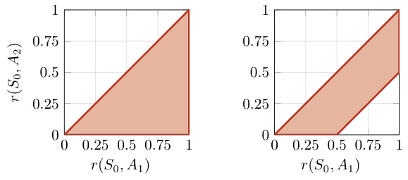
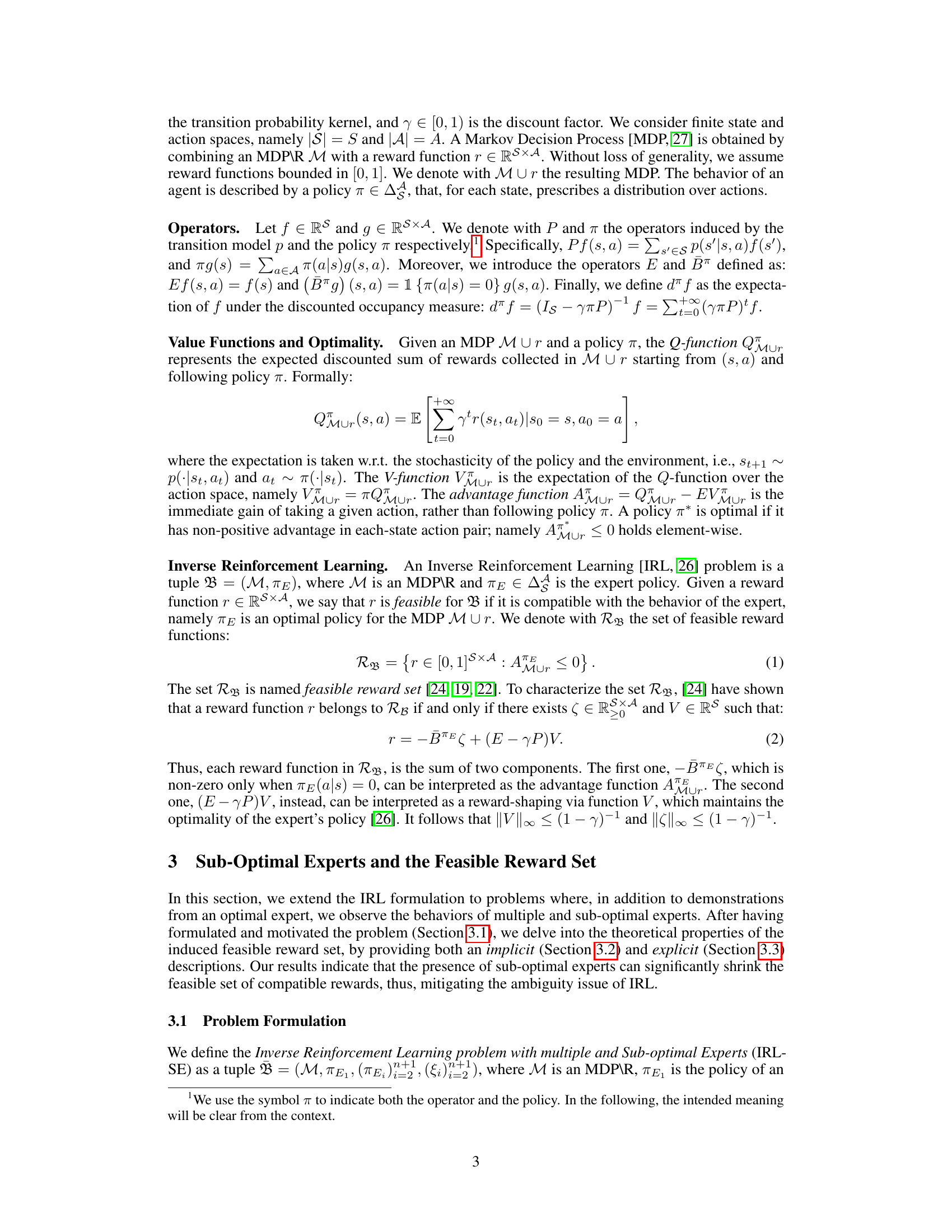
🔼 This figure visualizes the feasible reward sets for single-expert and multiple sub-optimal expert Inverse Reinforcement Learning (IRL) problems. The left panel shows the feasible reward set for a single optimal expert. The right panel shows the significantly reduced feasible reward set when incorporating a sub-optimal expert with a sub-optimality bound ξi = 0.5. The reduction demonstrates how additional data from sub-optimal experts can mitigate the inherent ambiguity in IRL.
read the caption
Figure 2: Visualization of the feasible reward set (i.e., shaded red area) for the problems described in Example 3.5. On the left, the feasible reward set for the single-expert IRL problem and on the right the feasible reward set for the multiple and sub-optimal setting when using ξi = 0.5.
🔼 This figure shows a simple Markov Decision Process (MDP) with two states (S₀ and S₁) and two experts (an optimal expert and a sub-optimal expert). The optimal expert’s policy (πE₁) is deterministic, always selecting action A₁ from state S₀ and action A from state S₁. The sub-optimal expert (πEᵢ) has the same policy as the optimal expert in state S₁, but its policy differs in state S₀. The figure highlights the use of sub-optimal expert demonstrations in inverse reinforcement learning (IRL). By including data from both experts, it becomes easier to determine the reward function that best represents the intentions of the optimal expert, as the sub-optimal expert’s actions provide additional constraints on the feasible reward set. This reduces the inherent ambiguity in IRL, especially in real-world scenarios where human experts show varying skill levels.
read the caption
Figure 1: MDP example, with 2 states and 2 experts, that highlights the benefits of sub-optimal experts (Example 3.5). In S₁ both πE₁ and πEᵢ are identical, i.e., πE₁ (A|S₁) = πEᵢ (A|S₁) = 1.

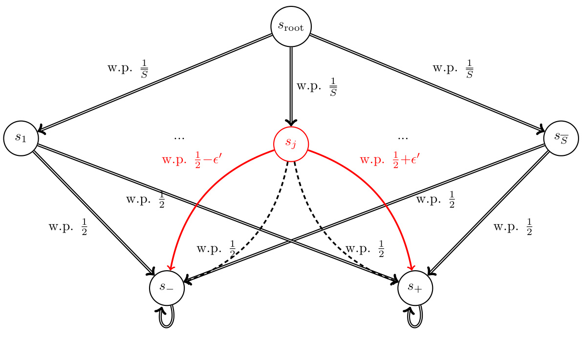
🔼 This figure is a graphical representation of a Markov Decision Process (MDP) used in the proof of Theorem E.2 within Section 4.2 of the paper. The MDP has a root node (Sroot) and two branches leading to distinct subtrees, representing different sets of states (S1 to S5). Each subtree has a terminal state (S− and S+). The solid and dashed lines represent different transition probabilities from an intermediate state (Si) to terminal nodes (S− and S+) depending on the actions taken (Aj). The key aspect illustrated is that the transition probabilities are manipulated to create variations within the feasible reward set which is central to the statistical complexity analysis presented in the theorem.
read the caption
Figure 3: Representation of the IRL-SE problem for the instances used in Theorem E.2.

🔼 This figure illustrates an example MDP used in the proof of Theorem E.4, which focuses on lower-bounding the sample complexity of identifying feasible reward functions in the presence of suboptimal experts. The MDP has states {s_root, s_1, …, s_S, s_sink}, where s_root is the start state, s_1…s_S are intermediate states, and s_sink is the terminal state. The optimal expert always chooses action a1, while the suboptimal expert chooses action a2 with probability π_min in states s_1…s_S. The structure and transition probabilities are designed to demonstrate the impact of having a suboptimal expert on the difficulty of learning the feasible reward set.
read the caption
Figure 5: Representation of the IRL-SE problem for the instances used in Theorem E.4.
🔼 This figure shows a comparison of feasible reward sets between single-expert IRL and multi-agent IRL with suboptimal experts. The left panel shows the feasible reward set for a single optimal expert, while the right panel shows the feasible reward set when incorporating a suboptimal expert with a suboptimality bound ξi = 0.5. The shaded red area represents the feasible reward set. The figure illustrates how the addition of suboptimal expert data reduces the ambiguity of inverse reinforcement learning by shrinking the feasible reward set.
read the caption
Figure 2: Visualization of the feasible reward set (i.e., shaded red area) for the problems described in Example 3.5. On the left, the feasible reward set for the single-expert IRL problem and on the right the feasible reward set for the multiple and sub-optimal setting when using ξi = 0.5.
More on tables

🔼 This table lists the symbols and notations used throughout the paper. It includes mathematical notations, variable names, and set definitions relevant to the Inverse Reinforcement Learning problem with multiple and sub-optimal experts (IRL-SE), including the number of sub-optimal experts, policies, sub-optimality bounds, and various sets related to reward functions and their estimations.
read the caption
Table 1: Notation

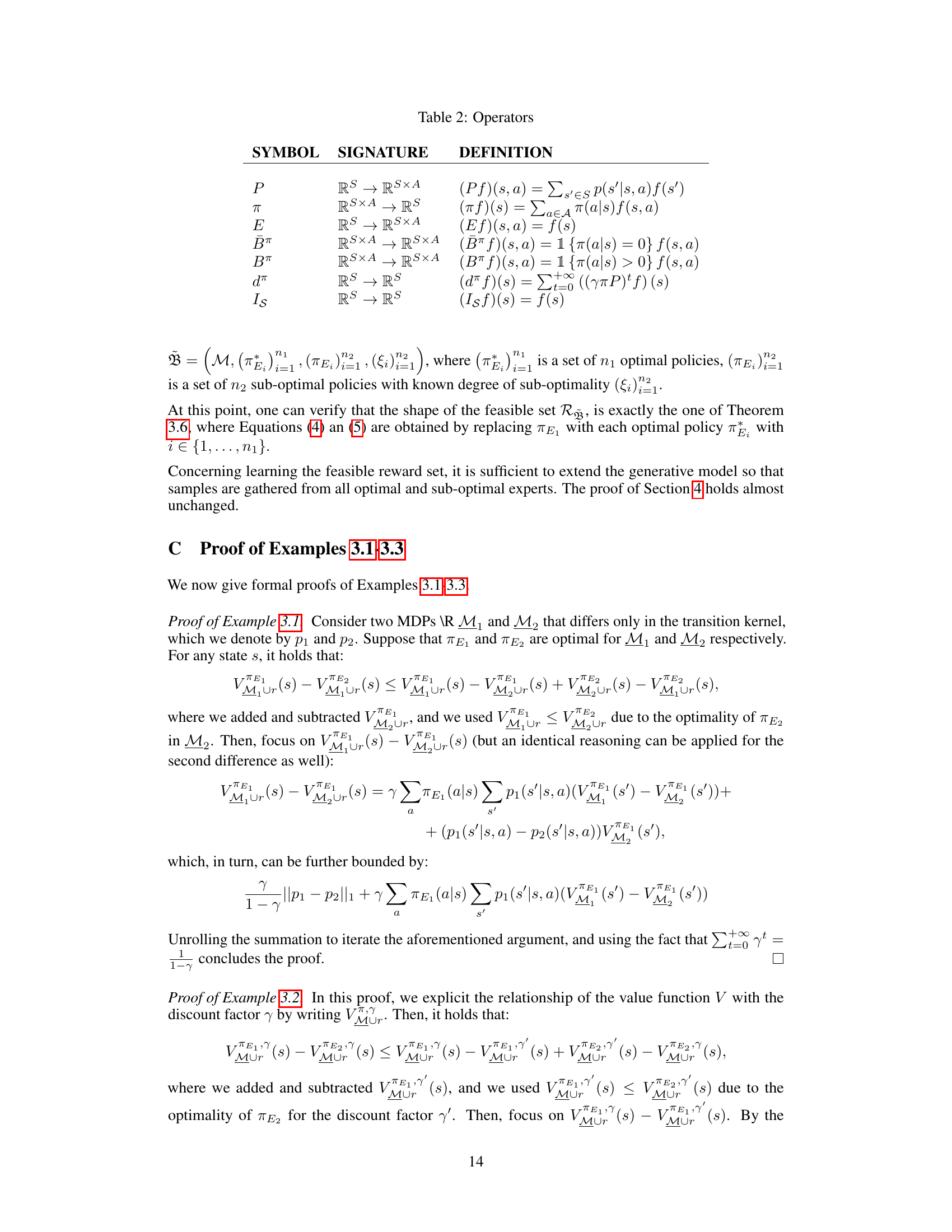
🔼 This table defines the operators used throughout the paper. The operators act on reward functions (RS or RSxA) and policies (π). For example, the ‘P’ operator represents the Bellman expectation operator for the transition probability kernel. ‘π’ is the policy operator, ‘E’ extracts the state-based component of a state-action function, Bπ masks the action-value function for actions that have zero probability under the policy. B¬π is the complement of Bπ, selecting actions with non-zero policy probability. dπ is the discounted state occupancy measure, and IS is the identity operator on functions of the state space.
read the caption
Table 2: Operators
Full paper#

