TL;DR#
Multivariate time series forecasting is crucial across many domains, but existing methods struggle to balance channel independence (resistance to distribution drift) with channel correlation (capturing interdependencies). Many models use attention mechanisms, but these are computationally expensive and may over-rely on correlation, performing poorly under distribution shifts. Additionally, simpler channel-independent models ignore valuable information.
SOFTS introduces a novel MLP-based model that efficiently manages channel interactions through a centralized STAR (STar Aggregate-Redistribute) module. This avoids the quadratic complexity of distributed methods, offering linear complexity with respect to the number of channels and time steps, and improving robustness to noisy channels. Empirical results demonstrate that SOFTS outperforms other state-of-the-art models, showcasing its efficiency and effectiveness.
Key Takeaways#
Why does it matter?#
This paper is important because it introduces SOFTS, a novel and efficient MLP-based model for multivariate time series forecasting. It addresses the limitations of existing methods by efficiently capturing channel correlations without sacrificing efficiency or robustness. This offers a significant improvement to current forecasting techniques and opens avenues for further research into efficient and robust forecasting models. The STAR module introduced is also versatile and applicable to various forecasting models, extending the impact of the work beyond the proposed model itself.
Visual Insights#

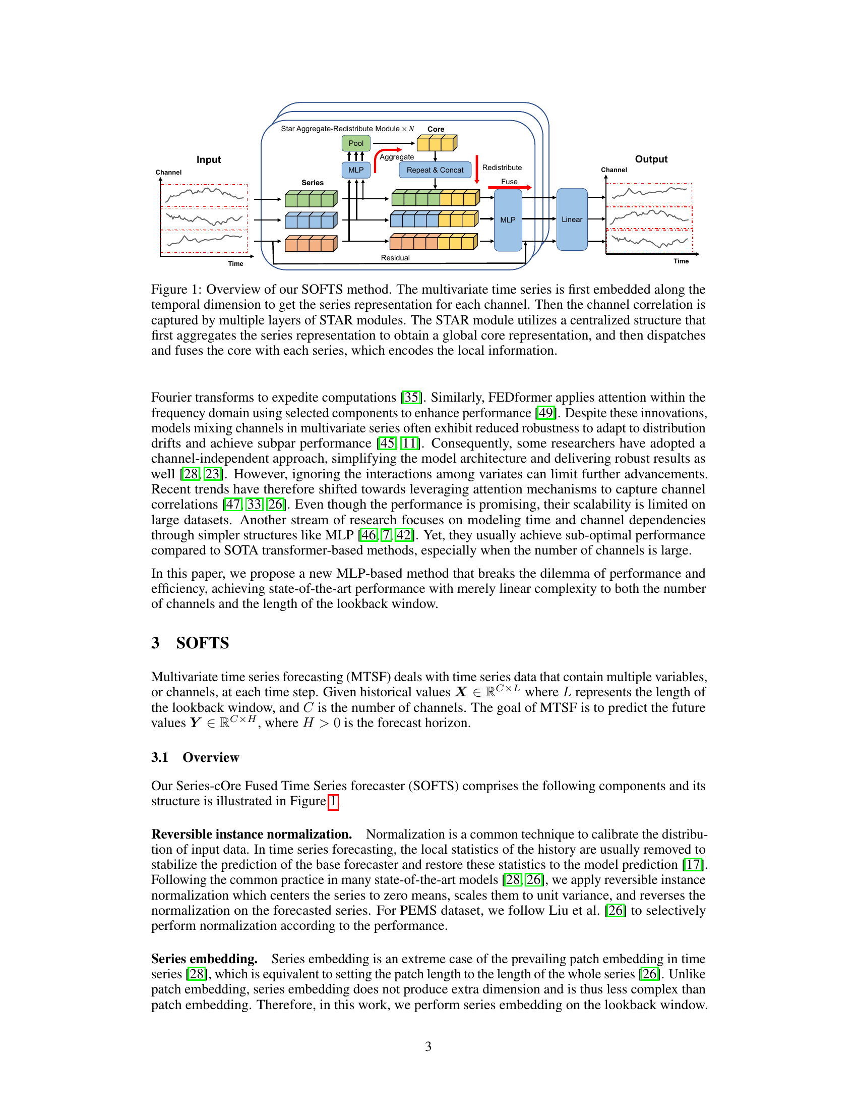
🔼 This figure illustrates the architecture of the Series-cOre Fused Time Series forecaster (SOFTS). The input is a multivariate time series, which is first embedded. Then, multiple STAR (STar Aggregate-Redistribute) modules process the data. Each STAR module uses a centralized strategy: it aggregates all series into a global core representation and then fuses this core with individual series representations to capture correlations effectively. Finally, a linear layer produces the forecast.
read the caption
Figure 1: Overview of our SOFTS method. The multivariate time series is first embedded along the temporal dimension to get the series representation for each channel. Then the channel correlation is captured by multiple layers of STAR modules. The STAR module utilizes a centralized structure that first aggregates the series representation to obtain a global core representation, and then dispatches and fuses the core with each series, which encodes the local information.

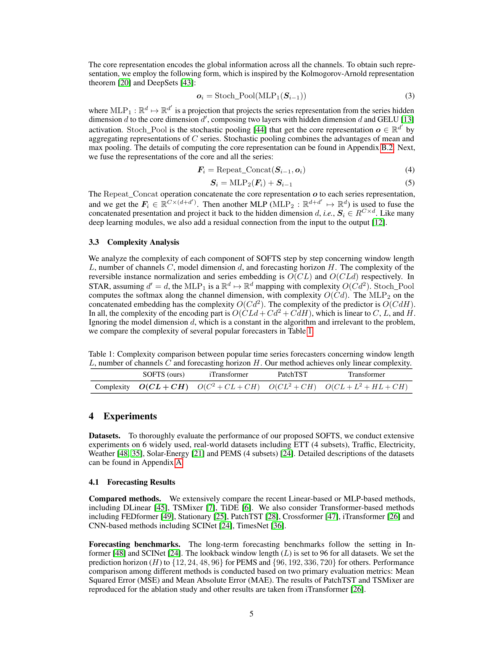
🔼 This table compares the computational complexity of several popular time series forecasting models, including the proposed SOFTS model. The complexity is expressed in terms of the window length (L), number of channels (C), and forecasting horizon (H). The table shows that SOFTS has a linear complexity, unlike other models which have quadratic or higher complexity. This highlights SOFTS’ efficiency, particularly when dealing with high-dimensional multivariate time series.
read the caption
Table 1: Complexity comparison between popular time series forecasters concerning window length L, number of channels C and forecasting horizon H. Our method achieves only linear complexity.
In-depth insights#
STAR Module Fusion#
The conceptualization of a ‘STAR Module Fusion’ within a multivariate time series forecasting model presents a compelling approach to efficiently capture channel interdependencies. The core innovation likely involves a centralized aggregation mechanism, where individual channel representations are combined into a global core, representing the collective behavior of the entire series. This core then acts as a conduit of information, being redistributed and fused with the individual channel representations to facilitate enhanced channel interactions. This centralized architecture offers advantages in terms of computational efficiency, scaling linearly instead of quadratically with the number of channels, unlike attention mechanisms. The effectiveness of this method hinges on the quality of the global core representation; a poorly constructed core could hinder performance. The broad applicability of the STAR module to other forecasting models is also a key aspect to evaluate, highlighting its potential as a generic module for enhancing various forecasting architectures.
MLP-Based Forecasting#
MLP-based forecasting methods offer a compelling alternative to complex transformer models for time series prediction. Their simplicity and computational efficiency are attractive, especially when dealing with high-dimensional or long time series data where transformers can become prohibitively expensive. However, achieving comparable accuracy to transformers often requires careful design choices, such as the incorporation of specialized modules to capture temporal dependencies and channel interactions effectively. The success of MLP-based approaches hinges on effectively leveraging the strengths of MLPs — their ability to learn non-linear relationships efficiently — while mitigating their limitations in handling long-range dependencies. Therefore, future research directions should explore novel architectural designs and training techniques to further bridge the performance gap with transformers while retaining the crucial advantages of simplicity and efficiency.
Efficiency & Scalability#
The efficiency and scalability of a model are critical factors determining its practical applicability, especially when dealing with large-scale datasets common in multivariate time series forecasting. Efficiency often refers to computational cost; a model’s ability to produce accurate predictions within reasonable time and resource constraints. Scalability, on the other hand, focuses on a model’s capacity to handle increasing data volume and complexity without a disproportionate rise in computational demands. A highly scalable model can adapt smoothly to datasets of growing size, maintaining performance and efficiency. This paper’s emphasis on achieving both efficiency and scalability is vital because it directly addresses the practical challenges inherent in large-scale time series analysis. The proposed method, with its linear time complexity, stands as a testament to this focus, suggesting broad applicability to diverse real-world problems where massive datasets are routinely encountered.
Channel Interaction#
The concept of ‘Channel Interaction’ in multivariate time series forecasting is crucial for enhancing predictive accuracy. Traditional methods often treated channels independently, neglecting valuable interdependencies. The challenge lies in effectively capturing these correlations without adding excessive computational complexity. Sophisticated attention mechanisms and mixer layers were explored, but they proved computationally expensive, especially with high-dimensional data. A novel approach involves a centralized strategy, aggregating information from all channels to form a global core representation, then redistributing this information back to individual channels to facilitate interaction. This centralized approach offers a significant advantage in efficiency and scalability, reducing computational cost from quadratic to linear complexity. While improving efficiency, the method also needs to address the potential for the global representation to be less robust than the original individual channels to anomalies. Therefore, careful consideration of aggregation and redistribution strategies is critical to balance efficiency and robustness.
Future Research#
Future research directions for efficient multivariate time series forecasting (MTSF) should prioritize developing more robust core representation methods within the STAR module to ensure accuracy across diverse datasets and handle noisy or missing data effectively. Exploring alternative aggregation and redistribution strategies beyond the centralized STAR approach could significantly enhance performance and scalability. The inherent limitations of MLP-based models necessitate investigating hybrid architectures that combine the strengths of MLPs with advanced techniques such as transformers or graph neural networks for improved long-term dependency modeling and increased robustness to distribution shifts. Finally, rigorous empirical evaluations on a wider range of real-world datasets, encompassing varying data characteristics and noise levels, are essential to validate the generalizability and practical applicability of proposed advancements in MTSF. The development of techniques for handling imbalanced datasets and those with non-stationary properties remain vital areas for future work.
More visual insights#
More on figures
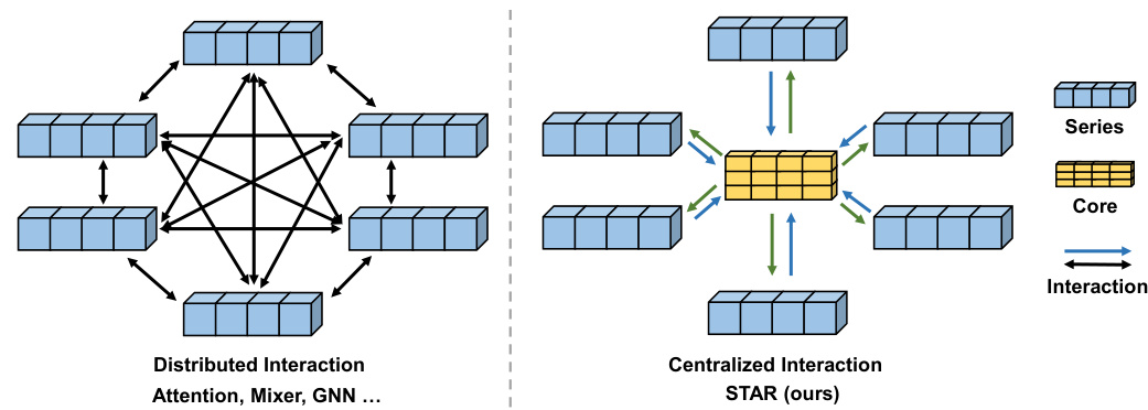
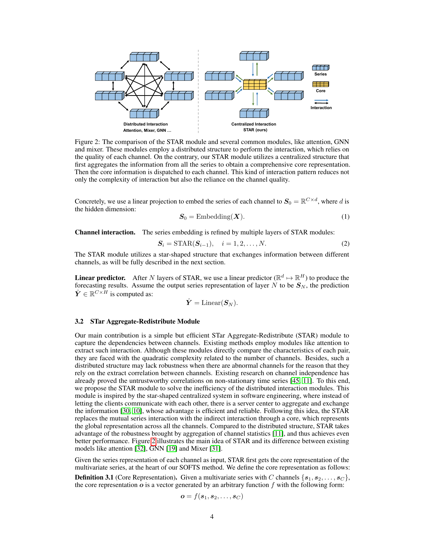
🔼 This figure compares the STAR module with other common interaction methods like attention, GNN, and mixer. The traditional methods use a distributed approach, where each channel interacts directly with others, leading to high complexity and dependence on individual channel quality. In contrast, STAR uses a centralized approach. It first aggregates information from all channels into a ‘core’ representation. Then, this core is fused with each individual channel’s representation to facilitate indirect interaction between channels. This significantly reduces complexity and makes the model less reliant on the reliability of individual channels.
read the caption
Figure 2: The comparison of the STAR module and several common modules, like attention, GNN and mixer. These modules employ a distributed structure to perform the interaction, which relies on the quality of each channel. On the contrary, our STAR module utilizes a centralized structure that first aggregates the information from all the series to obtain a comprehensive core representation. Then the core information is dispatched to each channel. This kind of interaction pattern reduces not only the complexity of interaction but also the reliance on the channel quality.
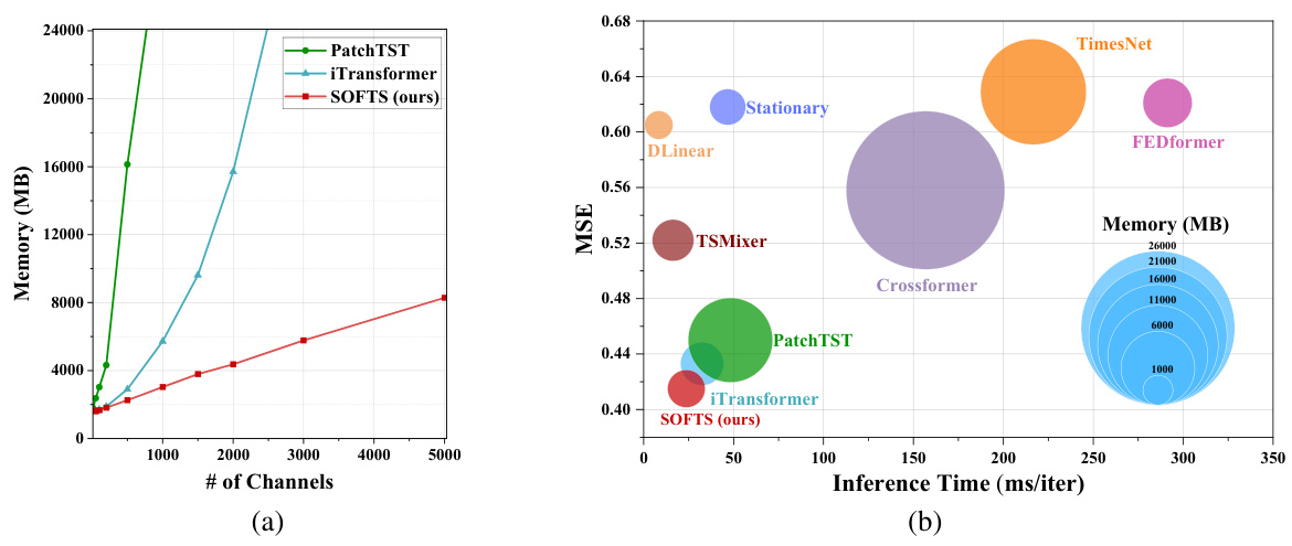
🔼 This figure compares the memory and inference time of several time series forecasting models, including SOFTS, on datasets with varying numbers of channels. Part (a) shows how memory usage increases with the number of channels for different models; SOFTS demonstrates significantly better scalability compared to transformer-based models like PatchTST and iTransformer. Part (b) shows a scatter plot comparing inference time and memory usage; SOFTS is significantly more efficient and less memory-intensive than most other methods. The superior efficiency of SOFTS is particularly pronounced when the number of channels is high.
read the caption
Figure 3: Memory and time consumption of different models. In Figure 3a, we set the lookback window L = 96, horizon H = 720, and batch size to 16 in a synthetic dataset we conduct. In Figure 3b, we set the lookback window L = 96, horizon H = 720, and batch size to 4 in Traffic dataset. Figure 3a reveals that SOFTS model scales to large number of channels more effectively than Transformer-based models. Figure 3b shows that previous Linear-based or MLP-based models such as DLinear and TSMixer perform poorly with a large number of channels. While SOFTS model demonstrates efficient performance with minimal memory and time consumption.

🔼 This figure compares the memory and time consumption of different time series forecasting models, including SOFTS, on the Traffic dataset. Figure 3a demonstrates that SOFTS scales more effectively to a large number of channels compared to Transformer-based models. Figure 3b illustrates the generally poor performance of linear and MLP-based models when dealing with many channels, highlighting the efficiency of SOFTS.
read the caption
Figure 3: Memory and time consumption of different models. In Figure 3a, we set the lookback window L = 96, horizon H = 720, and batch size to 16 in a synthetic dataset we conduct. In Figure 3b, we set the lookback window L = 96, horizon H = 720, and batch size to 4 in Traffic dataset. Figure 3a reveals that SOFTS model scales to large number of channels more effectively than Transformer-based models. Figure 3b shows that previous Linear-based or MLP-based models such as DLinear and TSMixer perform poorly with a large number of channels. While SOFTS model demonstrates efficient performance with minimal memory and time consumption.

🔼 This figure compares the memory and time usage of different time series forecasting models, specifically highlighting the efficiency of SOFTS. Part (a) shows that SOFTS’s memory usage scales linearly with the number of channels, unlike others. Part (b) demonstrates SOFTS’s superior speed and lower memory consumption compared to other models, especially when dealing with many channels.
read the caption
Figure 3: Memory and time consumption of different models. In Figure 3a, we set the lookback window L = 96, horizon H = 720, and batch size to 16 in a synthetic dataset we conduct. In Figure 3b, we set the lookback window L = 96, horizon H = 720, and batch size to 4 in Traffic dataset. Figure 3a reveals that SOFTS model scales to large number of channels more effectively than Transformer-based models. Figure 3b shows that previous Linear-based or MLP-based models such as DLinear and TSMixer perform poorly with a large number of channels. While SOFTS model demonstrates efficient performance with minimal memory and time consumption.

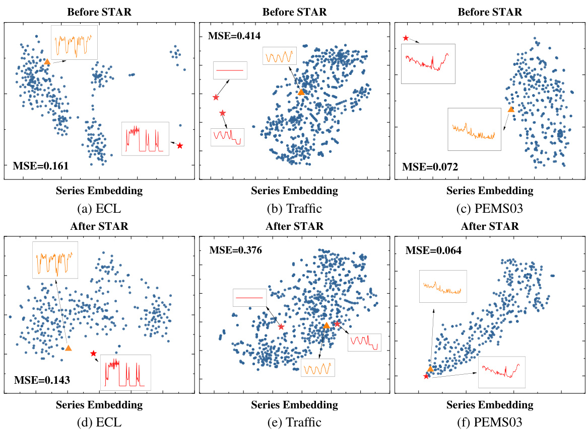
🔼 This figure compares the series embeddings before and after applying the STAR module. It shows that the STAR module helps cluster abnormal channels (with unusual characteristics) closer to the normal channels, improving prediction accuracy. The third subplot demonstrates the robustness of SOFTS against noise in a single channel.
read the caption
Figure 6: Figure 6a 6b: T-SNE of the series embeddings on the Traffic dataset. 6a: the series embeddings before STAR. Two abnormal channels (*) are located far from the other channels. Forecasting on the embeddings achieves 0.414 MSE. 6b: series embeddings after being adjusted by STAR. The two channels are clustered towards normal channels (△) by exchanging channel information. Adapted series embeddings improve forecasting performance to 0.376. Figure 6c: Impact of noise on one channel. Our method is more robust against channel noise than other methods.

🔼 This figure compares the memory usage and inference time of various time series forecasting models, including SOFTS, on the Traffic dataset with different numbers of channels. It highlights SOFTS’s superior efficiency in terms of both memory usage and inference time, especially when dealing with a high number of channels, unlike Transformer-based or simpler linear models.
read the caption
Figure 3: Memory and time consumption of different models. In Figure 3a, we set the lookback window L = 96, horizon H = 720, and batch size to 16 in a synthetic dataset we conduct. In Figure 3b, we set the lookback window L = 96, horizon H = 720, and batch size to 4 in Traffic dataset. Figure 3a reveals that SOFTS model scales to large number of channels more effectively than Transformer-based models. Figure 3b shows that previous Linear-based or MLP-based models such as DLinear and TSMixer perform poorly with a large number of channels. While SOFTS model demonstrates efficient performance with minimal memory and time consumption.

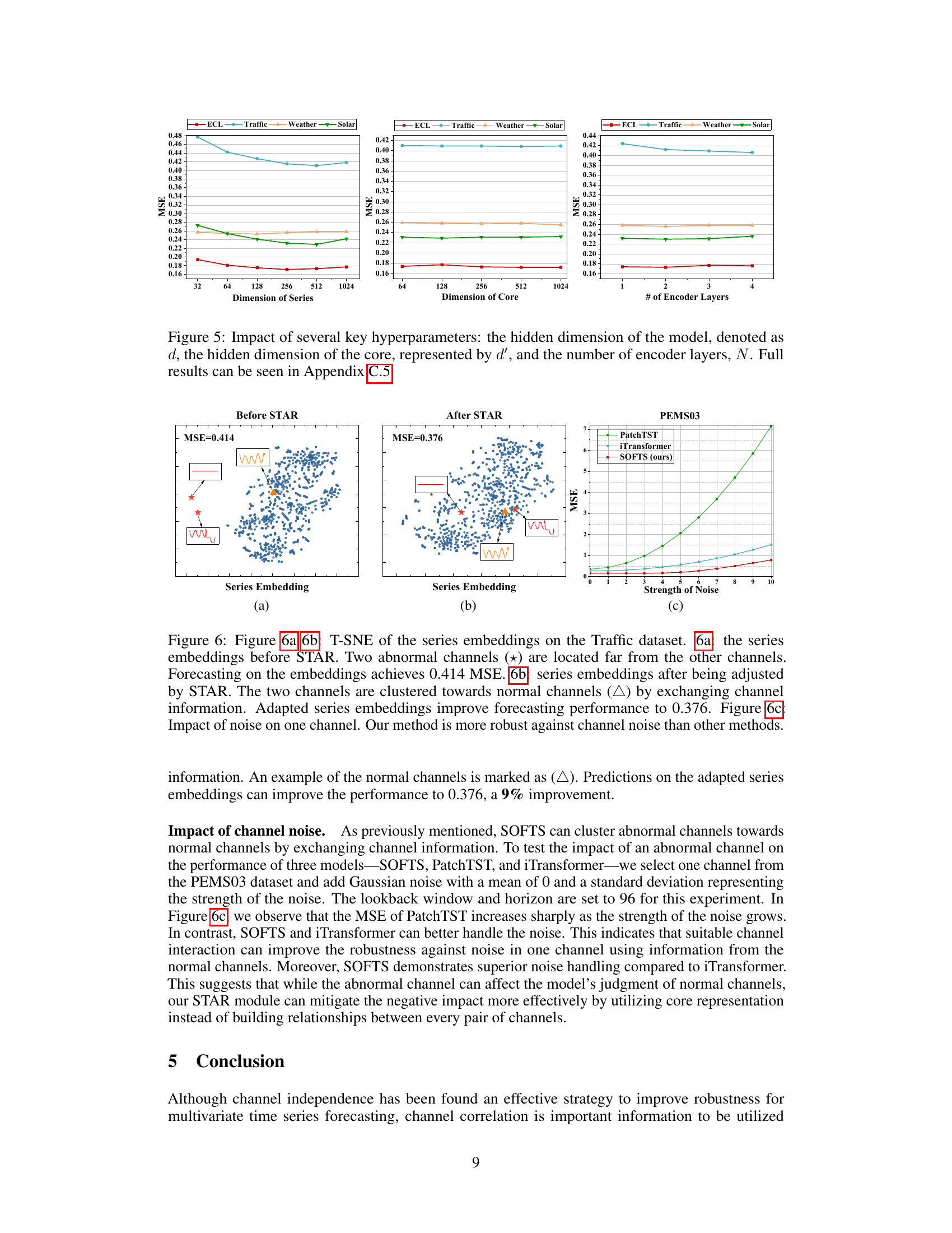
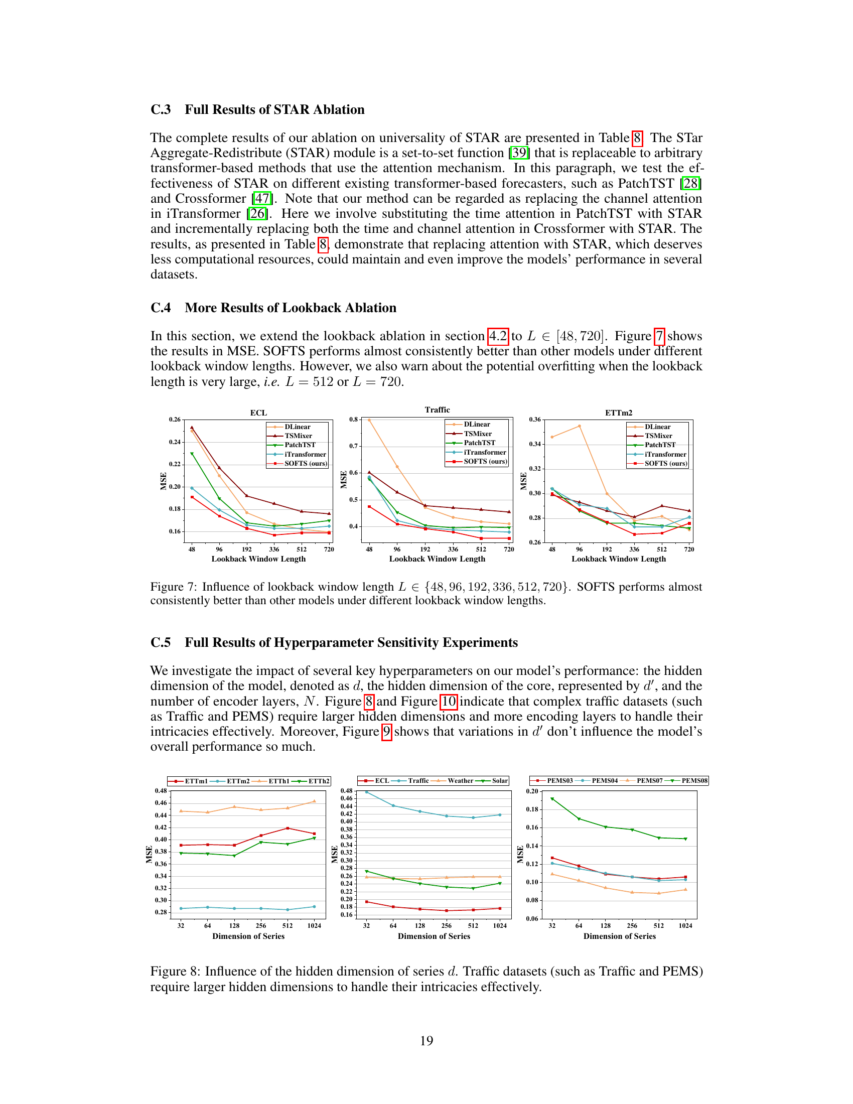
🔼 This figure shows the impact of three hyperparameters on the model’s performance: the hidden dimension of the model (d), the hidden dimension of the core (d’), and the number of encoder layers (N). The results are presented for six different datasets (ETTm1, ETTm2, ETTh1, ETTh2, ECL, Traffic, Weather, Solar, PEMS03, PEMS04, PEMS07, PEMS08). It demonstrates how these hyperparameters affect the model’s mean squared error (MSE) and indicates that more complex datasets might need larger values for these hyperparameters to achieve optimal results. Appendix C.5 contains the full results.
read the caption
Figure 5: Impact of several key hyperparameters: the hidden dimension of the model, denoted as d, the hidden dimension of the core, represented by d', and the number of encoder layers, N. Full results can be seen in Appendix C.5.

🔼 This figure illustrates the architecture of the Series-cOre Fused Time Series forecaster (SOFTS). The input is a multivariate time series. Each channel of the series is independently embedded. Then, the channel correlations are captured using multiple Star Aggregate-Redistribute (STAR) modules. Each STAR module aggregates series representations to form a global core representation, which is then fused with individual series representations. This process is repeated multiple times. Finally, a linear layer predicts the future values.
read the caption
Figure 1: Overview of our SOFTS method. The multivariate time series is first embedded along the temporal dimension to get the series representation for each channel. Then the channel correlation is captured by multiple layers of STAR modules. The STAR module utilizes a centralized structure that first aggregates the series representation to obtain a global core representation, and then dispatches and fuses the core with each series, which encodes the local information.

🔼 This figure shows the architecture of the Series-cOre Fused Time Series forecaster (SOFTS) model. The input is a multivariate time series. Each channel of the series is processed independently to obtain its series representation. Then, a novel STar Aggregate-Redistribute (STAR) module processes the representations from all channels to capture the correlations between them efficiently. The STAR module uses a centralized approach by aggregating all series into a global core representation, then redistributing and fusing this core with the individual series representations. Finally, a linear layer predicts the future values. This design allows SOFTS to achieve superior performance while maintaining only linear complexity.
read the caption
Figure 1: Overview of our SOFTS method. The multivariate time series is first embedded along the temporal dimension to get the series representation for each channel. Then the channel correlation is captured by multiple layers of STAR modules. The STAR module utilizes a centralized structure that first aggregates the series representation to obtain a global core representation, and then dispatches and fuses the core with each series, which encodes the local information.

🔼 The figure visualizes the core representation learned by the SOFTS model. The red line represents the core, which captures the global trend across all input channels. The other lines represent the original time series data for each channel. To create this visualization, the authors used a trained SOFTS model to extract series embeddings from the last encoder layer. Then they trained a two-layer MLP autoencoder to map these embeddings back to the original time series. This allows them to effectively visualize the core representation alongside the individual channel data.
read the caption
Figure 11: Visualization of the core, represented by the red line, alongside the original input channels. We freeze our model and extract the series embeddings from the last encoder layer to train a two-layer MLP autoencoder. This autoencoder maps the embeddings back to the original series, allowing us to visualize the core effectively.

🔼 This figure presents a high-level overview of the SOFTS (Series-cOre Fused Time Series forecaster) model architecture. It shows how multivariate time series data is processed in a step-by-step manner. First, each channel of the input time series undergoes embedding, transforming the raw data into a more suitable representation for the model. Then, a novel module called STAR (STar Aggregate-Redistribute) is applied multiple times to capture correlations between different channels. This module employs a centralized strategy, aggregating information from all channels into a single ‘core’ representation, which is then distributed back to individual channels to enhance their representations. Finally, a fusion process combines the refined channel representations, and a linear layer produces the final forecast result.
read the caption
Figure 1: Overview of our SOFTS method. The multivariate time series is first embedded along the temporal dimension to get the series representation for each channel. Then the channel correlation is captured by multiple layers of STAR modules. The STAR module utilizes a centralized structure that first aggregates the series representation to obtain a global core representation, and then dispatches and fuses the core with each series, which encodes the local information.

🔼 This figure presents a detailed overview of the SOFTS model’s architecture. The input is a multivariate time series. Each channel’s time series data is first embedded. Then, multiple STAR (STar Aggregate-Redistribute) modules process the data, capturing correlations between channels using a centralized aggregation and redistribution strategy. This differs from traditional methods that use distributed approaches like attention mechanisms. Finally, a linear layer produces the predicted future values.
read the caption
Figure 1: Overview of our SOFTS method. The multivariate time series is first embedded along the temporal dimension to get the series representation for each channel. Then the channel correlation is captured by multiple layers of STAR modules. The STAR module utilizes a centralized structure that first aggregates the series representation to obtain a global core representation, and then dispatches and fuses the core with each series, which encodes the local information.

🔼 This figure presents a schematic overview of the SOFTS model architecture. The input is a multivariate time series, which is processed in a series of steps. First, each channel of the time series is embedded along the time dimension, creating a series representation for each channel. Second, channel correlation is captured using multiple layers of the proposed STAR (STar Aggregate-Redistribute) module. The STAR module uses a centralized approach: it aggregates all series representations into a global core representation, then distributes and fuses this core back with the individual series representations. This fusion helps to effectively capture channel interactions. Finally, an MLP (Multilayer Perceptron) and a linear layer processes the combined representations to generate the final output, which represents the prediction.
read the caption
Figure 1: Overview of our SOFTS method. The multivariate time series is first embedded along the temporal dimension to get the series representation for each channel. Then the channel correlation is captured by multiple layers of STAR modules. The STAR module utilizes a centralized structure that first aggregates the series representation to obtain a global core representation, and then dispatches and fuses the core with each series, which encodes the local information.

🔼 This figure illustrates the architecture of the SOFTS model. It shows how multivariate time series data is processed through embedding, channel interaction (using STAR modules), and a linear predictor to generate predictions. The key element is the STAR (STar Aggregate-Redistribute) module, a centralized interaction mechanism for improved efficiency and robustness.
read the caption
Figure 1: Overview of our SOFTS method. The multivariate time series is first embedded along the temporal dimension to get the series representation for each channel. Then the channel correlation is captured by multiple layers of STAR modules. The STAR module utilizes a centralized structure that first aggregates the series representation to obtain a global core representation, and then dispatches and fuses the core with each series, which encodes the local information.
🔼 This figure provides a detailed overview of the SOFTS (Series-cOre Fused Time Series forecaster) model architecture. It illustrates the processing flow of multivariate time series data through several key stages: initial embedding, channel correlation capturing via STAR modules, and final prediction. The central component is the STAR module, which aggregates individual series representations into a global core representation, and then redistributes and fuses this core with individual series to efficiently capture channel interactions. The model is primarily MLP-based, aiming for efficiency and scalability.
read the caption
Figure 1: Overview of our SOFTS method. The multivariate time series is first embedded along the temporal dimension to get the series representation for each channel. Then the channel correlation is captured by multiple layers of STAR modules. The STAR module utilizes a centralized structure that first aggregates the series representation to obtain a global core representation, and then dispatches and fuses the core with each series, which encodes the local information.

🔼 This figure shows the architecture of the SOFTS model, a novel MLP-based model for multivariate time series forecasting. The model consists of three main components: series embedding, STAR modules, and a linear predictor. The input is a multivariate time series, and each channel is first embedded along the temporal dimension. The STAR (STar Aggregate-Redistribute) modules are the core of the model, aggregating the information from all channels to form a global representation (core) before redistributing and fusing it with each channel’s representation. This process is repeated for multiple layers of STAR modules to capture channel correlations efficiently. Finally, a linear predictor produces the forecasts.
read the caption
Figure 1: Overview of our SOFTS method. The multivariate time series is first embedded along the temporal dimension to get the series representation for each channel. Then the channel correlation is captured by multiple layers of STAR modules. The STAR module utilizes a centralized structure that first aggregates the series representation to obtain a global core representation, and then dispatches and fuses the core with each series, which encodes the local information.

🔼 This figure provides a detailed overview of the SOFTS model architecture. The input is a multivariate time series. Each channel of the time series is first processed via an embedding layer to produce a channel-specific representation. These representations are then fed into multiple STAR (STar Aggregate-Redistribute) modules. The STAR module is a core component that uses a centralized approach, aggregating information from all channels to generate a global core representation. This core representation is then combined (fused) with the individual channel representations. The fused representations are further processed through multiple MLP (multi-layer perceptron) layers and finally a linear layer before producing the forecast output. The design of the STAR module is key to the efficiency of the method.
read the caption
Figure 1: Overview of our SOFTS method. The multivariate time series is first embedded along the temporal dimension to get the series representation for each channel. Then the channel correlation is captured by multiple layers of STAR modules. The STAR module utilizes a centralized structure that first aggregates the series representation to obtain a global core representation, and then dispatches and fuses the core with each series, which encodes the local information.
More on tables
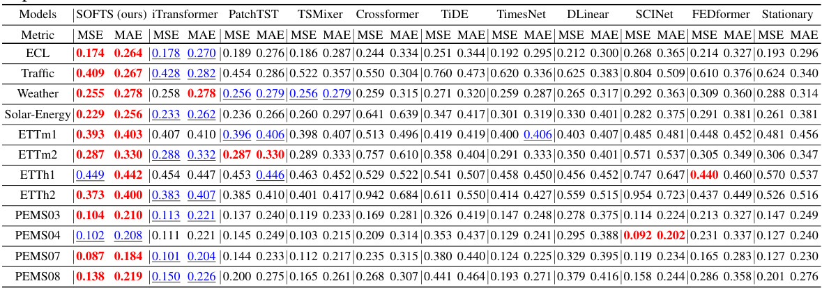
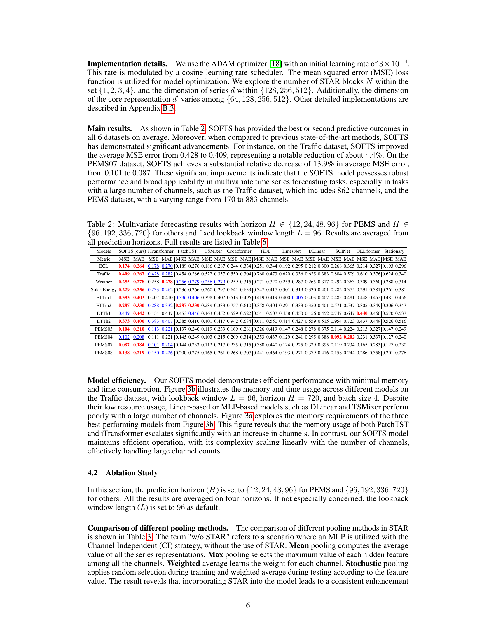
🔼 This table presents the results of multivariate time series forecasting experiments using various models, including the proposed SOFTS model. The table shows the Mean Squared Error (MSE) and Mean Absolute Error (MAE) achieved by each model on multiple datasets with varying prediction horizons (H) and a fixed lookback window length (L=96). The results are averaged across different prediction horizons for a more concise overview. Detailed results for each individual prediction horizon can be found in Table 6.
read the caption
Table 2: Multivariate forecasting results with horizon Η ∈ {12, 24, 48, 96} for PEMS and H∈ {96, 192, 336, 720} for others and fixed lookback window length L = 96. Results are averaged from all prediction horizons. Full results are listed in Table 6.

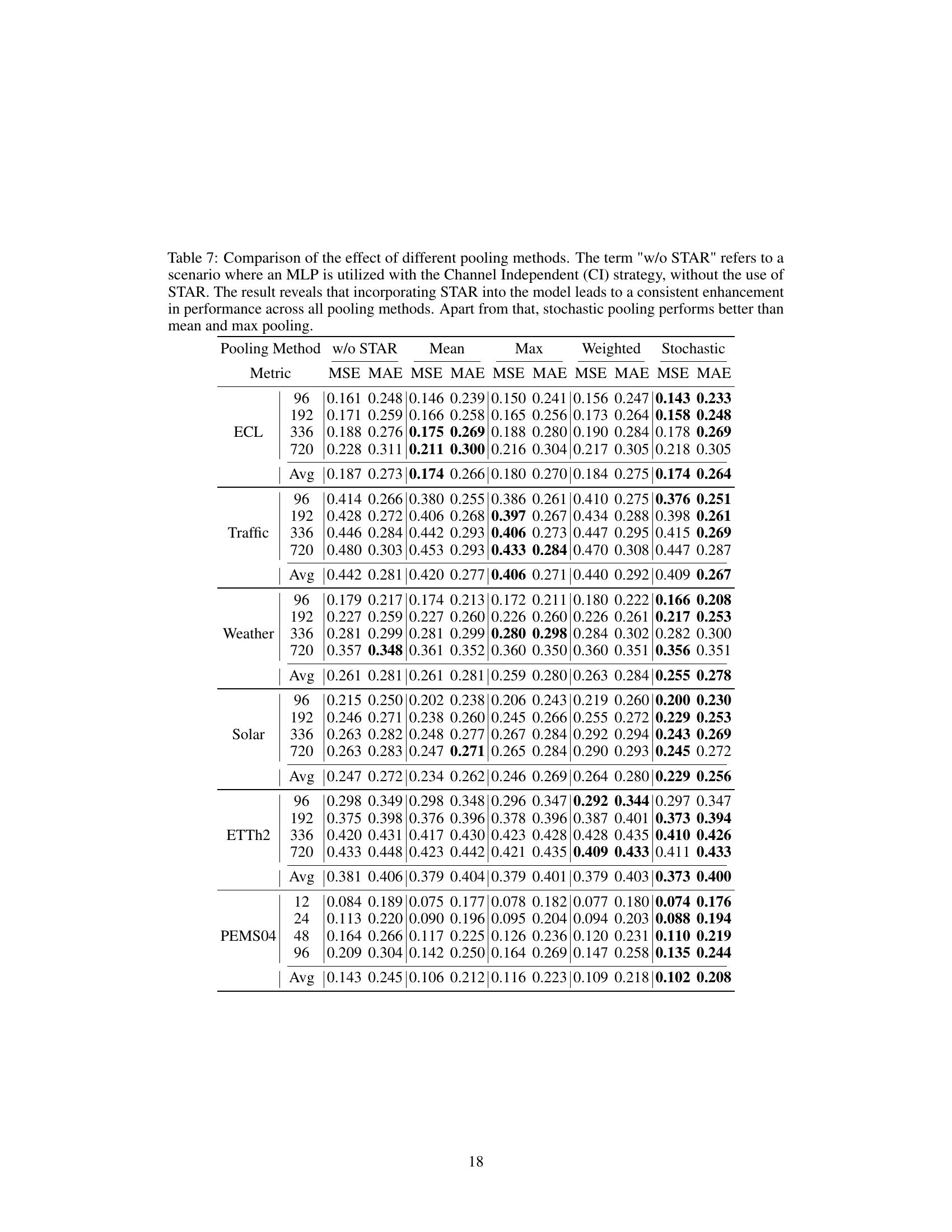
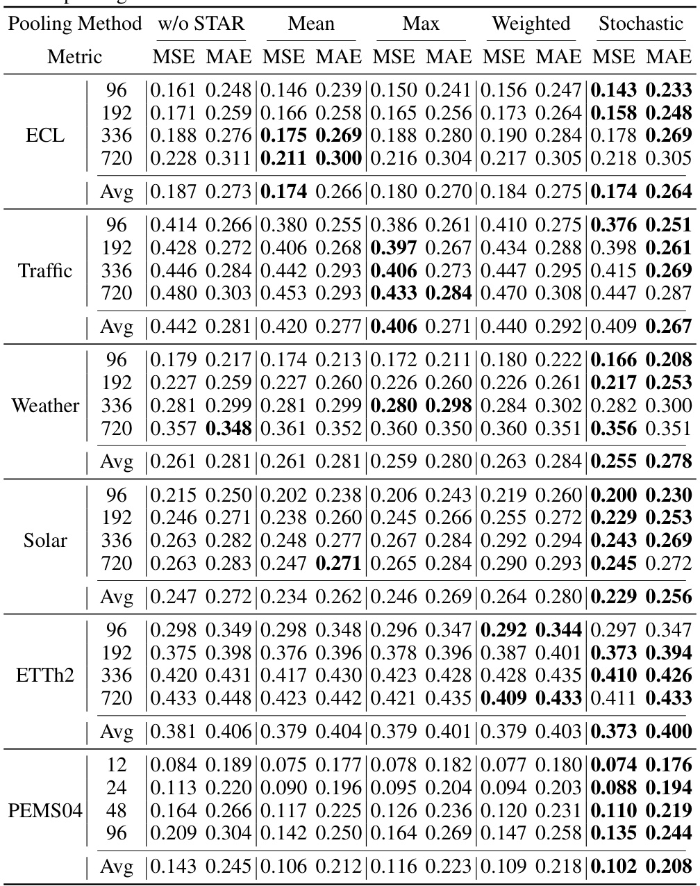
🔼 This table presents a comparison of different pooling methods used in the STAR module of the SOFTS model. It shows the Mean Squared Error (MSE) and Mean Absolute Error (MAE) achieved by using no STAR module (channel independence), mean pooling, max pooling, weighted average pooling, and stochastic pooling across six different datasets (ECL, Traffic, Weather, Solar, ETTh2, PEMS04). The results demonstrate that the STAR module consistently improves performance regardless of the pooling method used, with stochastic pooling generally performing the best.
read the caption
Table 7: Comparison of the effect of different pooling methods. The term 'w/o STAR' refers to a scenario where an MLP is utilized with the Channel Independent (CI) strategy, without the use of STAR. The result reveals that incorporating STAR into the model leads to a consistent enhancement in performance across all pooling methods. Apart from that, stochastic pooling performs better than mean and max pooling.

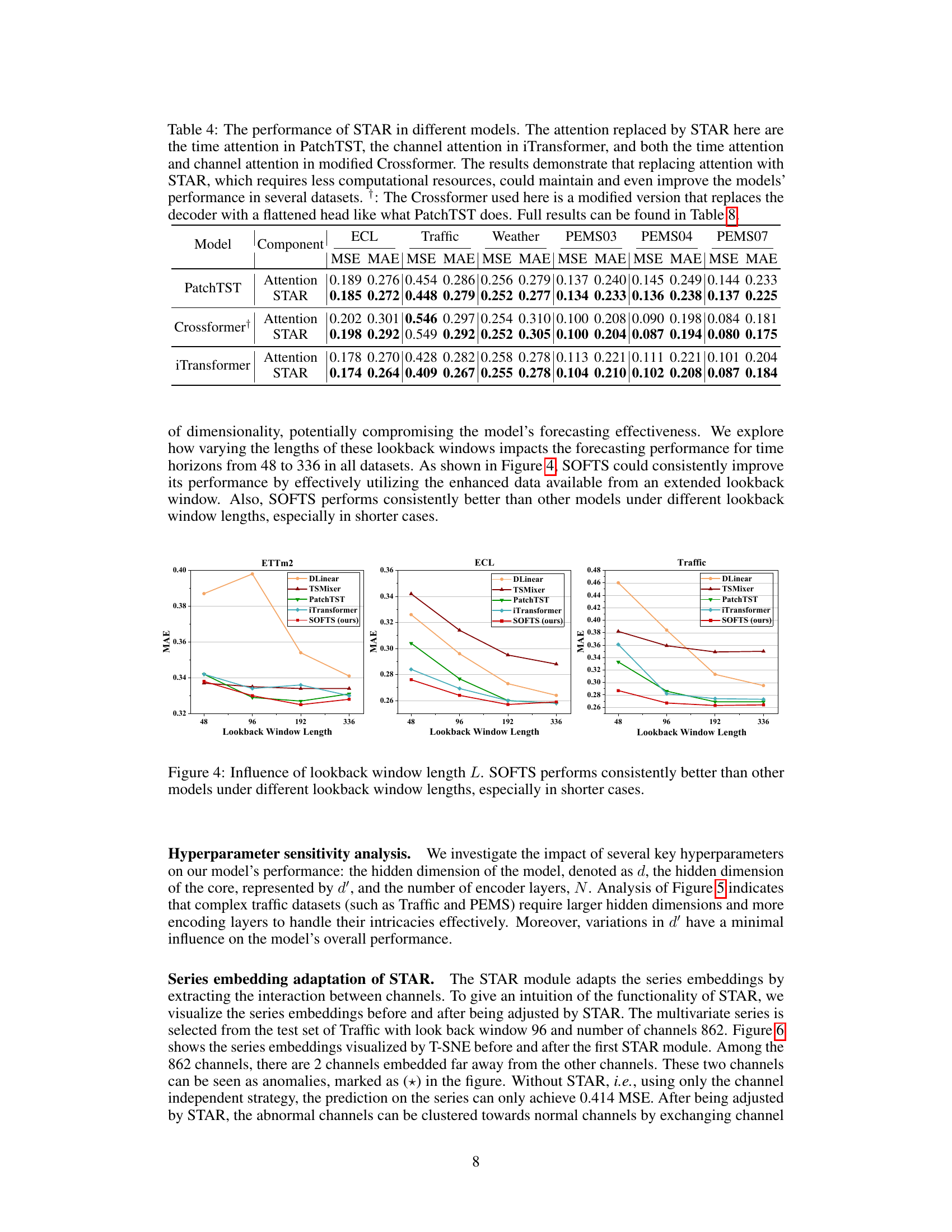
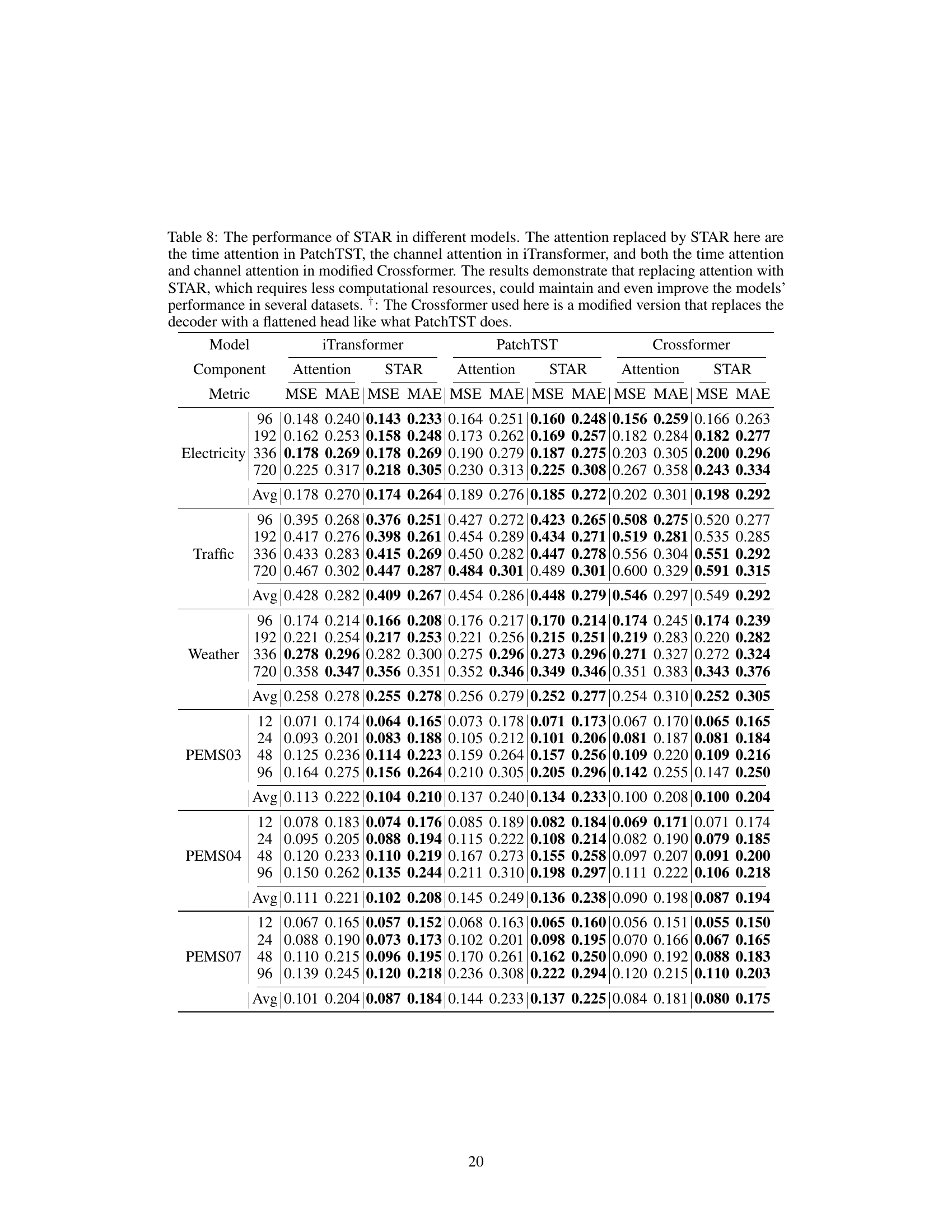
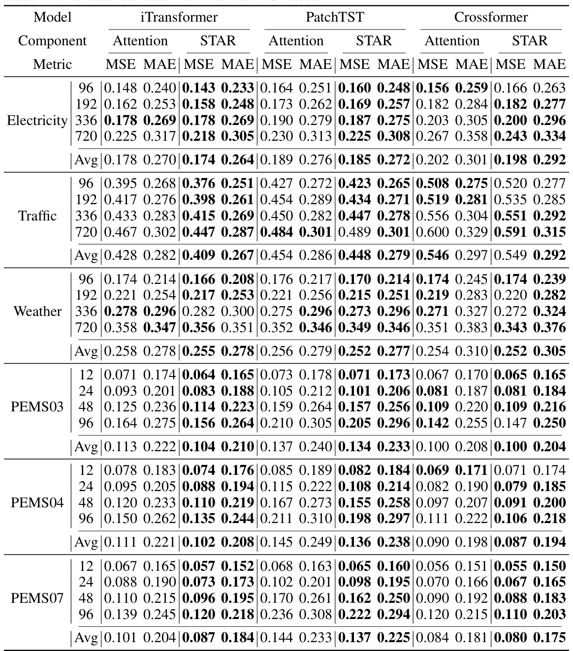
🔼 This table presents the results of an ablation study on the universality of the STAR module. The study replaced the attention mechanisms in three different transformer-based models (PatchTST, iTransformer, and Crossformer) with the STAR module. The table shows that using STAR, which is less computationally expensive, maintains or improves the performance of the models on several datasets.
read the caption
Table 8: The performance of STAR in different models. The attention replaced by STAR here are the time attention in PatchTST, the channel attention in iTransformer, and both the time attention and channel attention in modified Crossformer. The results demonstrate that replacing attention with STAR, which requires less computational resources, could maintain and even improve the models' performance in several datasets. †: The Crossformer used here is a modified version that replaces the decoder with a flattened head like what PatchTST does.

🔼 This table presents the performance comparison of the proposed SOFTS model with other state-of-the-art time series forecasting methods on six benchmark datasets (ETT, Traffic, Electricity, Weather, Solar-Energy, and PEMS). The table shows the mean squared error (MSE) and mean absolute error (MAE) for different prediction horizons (H) on each dataset. The lookback window length (L) is fixed at 96. Note that results for PatchTST and TSMixer are reproduced from previous studies, while other results are taken from iTransformer.
read the caption
Table 6: Multivariate forecasting results with prediction lengths H ∈ {12, 24, 48, 96} for PEMS and H ∈ {96, 192, 336, 720} for others and fixed lookback window length L = 96. The results of PatchTST and TSMixer are reproduced for the ablation study and other results are taken from iTransformer [26].

🔼 This table presents the results of multivariate time series forecasting experiments using various models, including the proposed SOFTS model. It shows the Mean Squared Error (MSE) and Mean Absolute Error (MAE) for multiple datasets across different prediction horizons (H). The lookback window length (L) is fixed at 96 for all experiments. The results are averaged across all prediction horizons for each dataset and model, with the complete results provided in Table 6. This table highlights the performance of SOFTS relative to state-of-the-art (SOTA) methods.
read the caption
Table 2: Multivariate forecasting results with horizon H ∈ {12, 24, 48, 96} for PEMS and H ∈ {96, 192, 336, 720} for others and fixed lookback window length L = 96. Results are averaged from all prediction horizons. Full results are listed in Table 6.
🔼 This table presents the average Mean Squared Error (MSE) and Mean Absolute Error (MAE) for various multivariate time series forecasting models, including the proposed SOFTS model, across six different datasets. The results are averaged across multiple prediction horizons (H) and use a fixed lookback window length (L=96). The table highlights the performance of SOFTS compared to state-of-the-art methods. Complete results for each individual prediction horizon are given in Table 6.
read the caption
Table 2: Multivariate forecasting results with horizon Η ∈ {12, 24, 48, 96} for PEMS and H∈ {96, 192, 336, 720} for others and fixed lookback window length L = 96. Results are averaged from all prediction horizons. Full results are listed in Table 6.
🔼 This table presents the results of multivariate time series forecasting experiments conducted on various datasets. It compares the performance of the proposed SOFTS model against several other state-of-the-art methods across different prediction horizons (H). The results are reported in terms of Mean Squared Error (MSE) and Mean Absolute Error (MAE), and include results using different lookback window lengths. Results from PatchTST and TSMixer were reproduced from previous research to enable comparison with the proposed SOFTS model.
read the caption
Table 6: Multivariate forecasting results with prediction lengths H ∈ {12, 24, 48, 96} for PEMS and H ∈ {96, 192, 336, 720} for others and fixed lookback window length L = 96. The results of PatchTST and TSMixer are reproduced for the ablation study and other results are taken from iTransformer [26].

🔼 This table presents the results of multivariate time series forecasting experiments conducted on various datasets using different forecasting models, including the proposed SOFTS model. The results are shown as Mean Squared Error (MSE) and Mean Absolute Error (MAE) for various prediction horizons. The table also includes a comparison with other state-of-the-art models for better context. The lookback window length was fixed at 96.
read the caption
Table 6: Multivariate forecasting results with prediction lengths H ∈ {12, 24, 48, 96} for PEMS and H ∈ {96, 192, 336, 720} for others and fixed lookback window length L = 96. The results of PatchTST and TSMixer are reproduced for the ablation study and other results are taken from iTransformer [26].
Full paper#

