TL;DR#
Training large deep neural networks is computationally expensive. A hardware-friendly approach to address this is N:M sparsity, where a subset of weights are non-zero in each group of weights. However, previous attempts using Straight-Through Estimators (STE) for 2:4 sparse pre-training suffer from optimization issues due to the discontinuous nature of the pruning functions. These issues lead to incorrect gradient descent, inability to predict descent amounts and sparse mask oscillations.
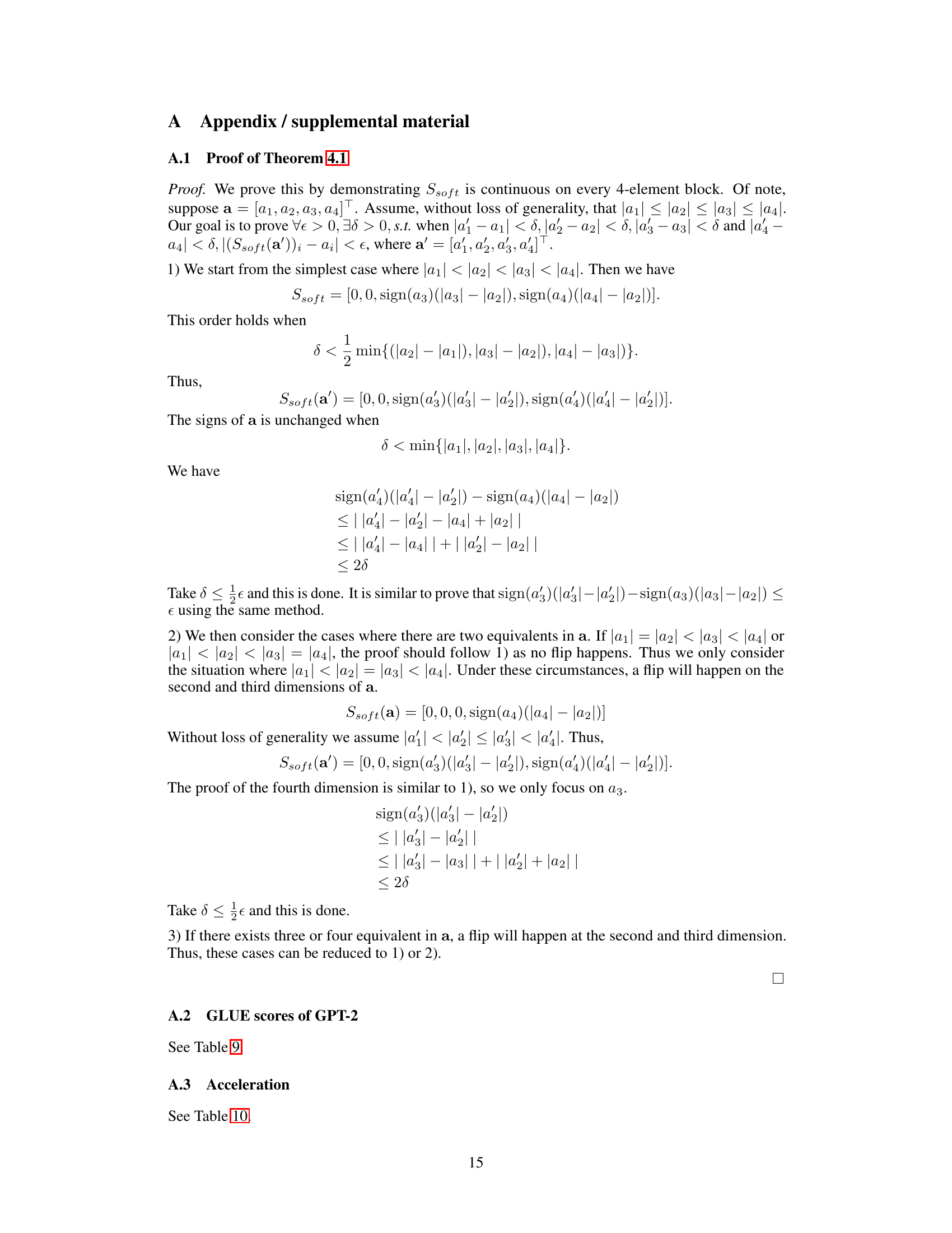
This paper introduces a new method, S-STE, to overcome the shortcomings of existing STE-based approaches. S-STE employs a continuous pruning function and fixed scaling factor to ensure smooth optimization. The authors use Minimum-Variance Unbiased Estimation for the activation gradient and leverage FP8 quantization for additional speedups. Experimental results show that S-STE outperforms existing 2:4 pre-training methods across various tasks, demonstrating improvements in both accuracy and efficiency and achieving results comparable to those of full-parameter models.
Key Takeaways#
Why does it matter?#
This paper is crucial for researchers working on efficient deep learning, particularly those focusing on sparse training and hardware acceleration. It directly addresses the limitations of existing sparse training methods, proposing a novel approach that significantly improves training speed and accuracy. The findings are relevant to current trends in reducing the computational cost of large-scale model training and offer new avenues for research on improving the optimization of sparse neural networks, opening doors for more efficient and sustainable AI development. The proposed S-STE method shows great promise for accelerating training of various models, including large-scale transformers, significantly lowering computational costs.
Visual Insights#
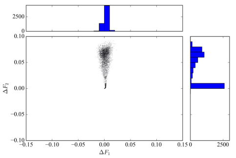
🔼 This figure shows a scatter plot of the change in objective function (ΔF₁) when updating both weights and masks versus the change in objective function (ΔF₂) when only updating weights. The data is from training a GPT-2 small 124M model for 6000 iterations. The marginal distributions of ΔF₁ and ΔF₂ are also shown as histograms. This figure is used to illustrate the phenomenon of incorrect descending direction in sparse training with hard thresholding.
read the caption
Figure 1: Scatter plot of AF₁ with AF₂ and their distributions on GPT-2 small 124M for iteration k∈ [1,6000].
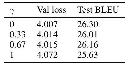
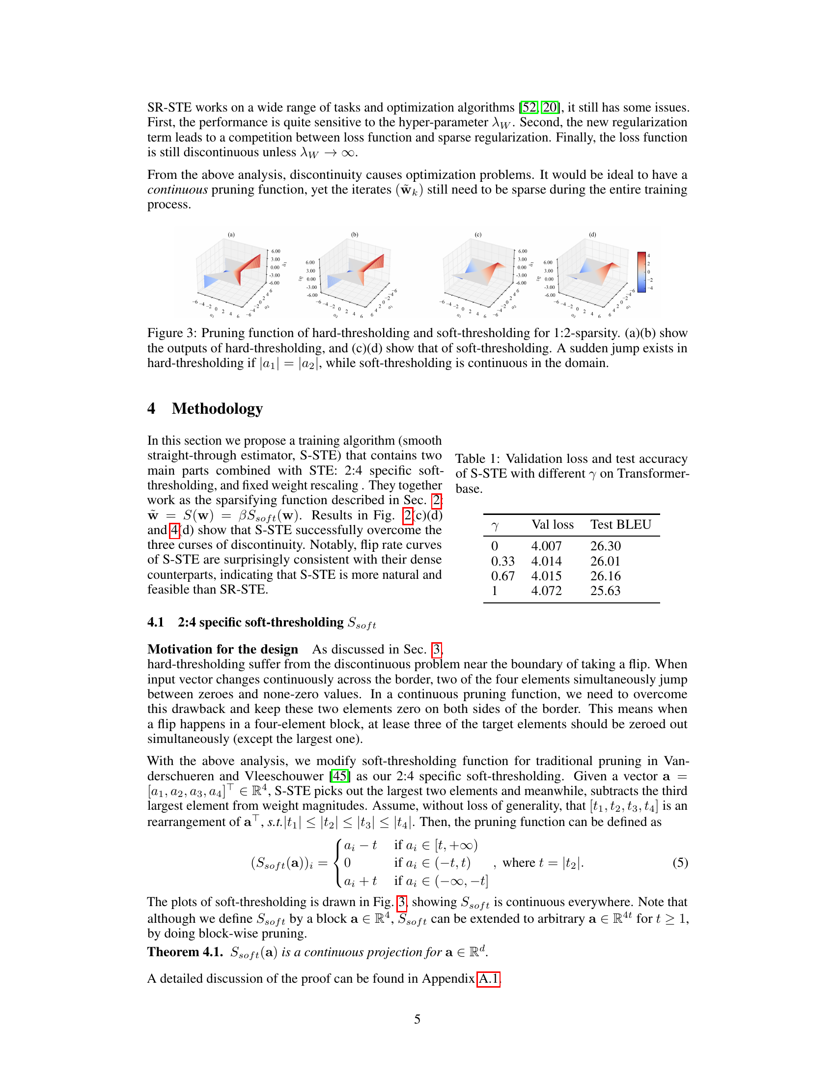
🔼 This table presents the results of experiments conducted using the S-STE method on a Transformer-base model. The experiment varied a hyperparameter, γ, and measured the resulting validation loss and test BLEU score. The table helps demonstrate the impact of this hyperparameter on model performance, allowing readers to determine the optimal γ value for this specific model and task.
read the caption
Table 1: Validation loss and test accuracy of S-STE with different γ on Transformer-base.
In-depth insights#
Sparse Training#
Sparse training, a crucial technique in deep learning, focuses on reducing the number of parameters in a neural network to enhance efficiency and reduce computational costs. Sparsity is achieved through various pruning methods, which selectively eliminate less important connections or neurons. This offers several advantages: it accelerates training and inference, lowers memory requirements, and can even improve generalization by mitigating overfitting. However, challenges remain: Simply removing weights can disrupt the network’s structure and hurt performance. Thus, effective sparse training demands sophisticated algorithms that carefully balance weight pruning with the need to maintain accuracy. Straight-through estimators (STE) and its variations are popular approaches, addressing the non-differentiability of hard thresholding pruning functions by approximating gradients. However, STE-based methods suffer from discontinuities leading to optimization issues. Recent work explores continuous pruning functions, aiming to overcome these challenges by smoothing the optimization landscape and enabling more stable training. The development of effective sparse training methods holds immense potential for deploying large-scale models on resource-constrained devices, making deep learning more accessible and sustainable.
S-STE Algorithm#
The hypothetical S-STE algorithm, as inferred from the context, is a novel approach to 2:4 sparse pre-training of neural networks. It addresses limitations of prior STE methods by introducing a continuous pruning function, eliminating the discontinuities that hinder optimization. This is achieved through a two-part process: a continuous projection of weights to achieve 2:4 sparsity, followed by rescaling of the sparse weights using a per-tensor fixed scaling factor. The algorithm also incorporates minimum-variance unbiased estimation for activation gradients and FP8 quantization to further boost efficiency. These combined innovations aim to overcome issues like incorrect descent direction, unpredictable descent amounts, and mask oscillation, leading to more stable and efficient training, potentially bridging the accuracy gap between sparse and dense pre-trained models. The continuity of the pruning function is a key innovation, allowing for smoother optimization and preventing abrupt changes in the sparse mask, ultimately enhancing training stability and performance.
Discontinuity Issues#
The concept of ‘Discontinuity Issues’ in the context of a research paper likely refers to problems arising from discontinuities in a system’s equations, algorithms, or processes. This is particularly relevant in areas like sparse neural network training, where discontinuous functions (e.g., hard thresholding for pruning weights) are employed. These discontinuities can lead to optimization difficulties, such as incorrect gradient descent directions, an inability to predict the magnitude of descent, and oscillations in the model’s parameters during training. Hard thresholding, a common technique, abruptly sets weights to zero, causing abrupt changes in the loss landscape. This makes it challenging for optimization algorithms to navigate efficiently, potentially leading to suboptimal solutions or convergence failure. Smooth approximations to these discontinuous functions are often explored as a potential solution to mitigate these issues, offering continuous optimization paths. The study of these discontinuities is crucial for designing effective training algorithms that leverage sparsity while avoiding the pitfalls of non-smooth behavior.
Optimization Analysis#
An optimization analysis of a sparse neural network training method would delve into the challenges posed by the discontinuous nature of traditional pruning functions. It would highlight how the discontinuous loss landscape leads to issues such as incorrect descent directions, an inability to predict the amount of descent, and oscillations in the sparse mask. A key aspect would involve exploring the impact of various optimization strategies, and comparing the performance of gradient-based methods, specifically stochastic gradient descent, when applied to both continuous and discontinuous pruning functions. The analysis should also cover the effects of different regularization techniques in stabilizing training and mitigating the challenges posed by discontinuities. Furthermore, a theoretical comparison of convergence properties for continuous versus discontinuous optimization schemes would provide critical insights. Finally, the analysis might discuss the computational trade-offs associated with different optimization approaches, considering the balance between speed and accuracy in the context of sparse training.
Future Directions#
Future research should explore extending S-STE’s applicability beyond linear layers to encompass attention mechanisms within transformer networks, demanding innovative dynamic sparse training strategies. Investigating alternative, smoother pruning functions could enhance continuity and mitigate potential discontinuities, improving optimization stability and accuracy. Further exploration is needed to fully leverage the potential of 2:4 sparsity by addressing limitations in the existing acceleration libraries for sparse matrix multiplications, aiming for more substantial speedups than currently observed. Finally, a thorough comparative analysis against other N:M sparse training methods under diverse model architectures and datasets is crucial to definitively establish S-STE’s superior performance and efficiency, especially in the context of large language models.
More visual insights#
More on figures

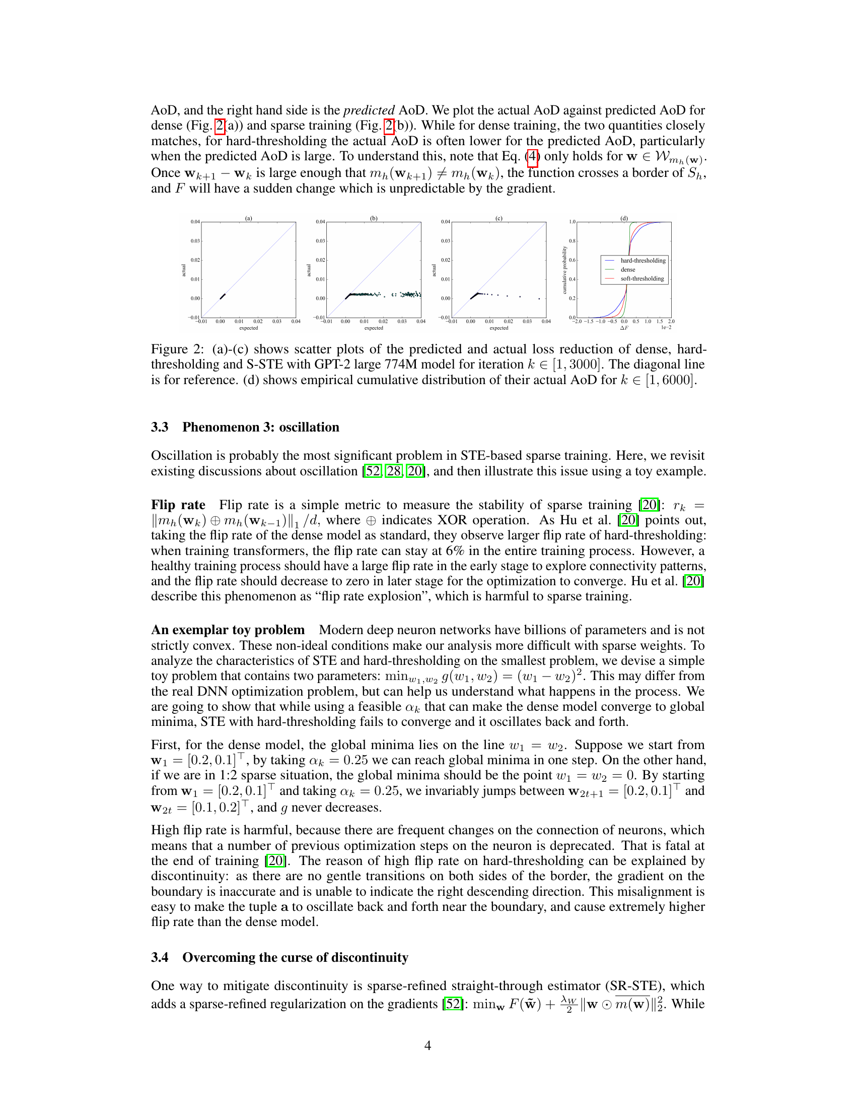
🔼 This figure compares the predicted and actual loss reduction for different training methods (dense, hard-thresholding, and S-STE) using the GPT-2 large 774M model. Subfigures (a), (b), and (c) show scatter plots illustrating the relationship between predicted and actual loss reduction for each method. The diagonal line represents perfect prediction. Subfigure (d) displays the cumulative distribution of the actual amount of descent (AoD) for each method, highlighting the differences in their optimization behavior.
read the caption
Figure 2: (a)-(c) shows scatter plots of the predicted and actual loss reduction of dense, hard-thresholding and S-STE with GPT-2 large 774M model for iteration k ∈ [1, 3000]. The diagonal line is for reference. (d) shows empirical cumulative distribution of their actual AoD for k ∈ [1, 6000].

🔼 This figure shows a comparison of the predicted and actual loss reduction for three different methods: dense training, hard-thresholding, and S-STE (smooth straight-through estimator). Subfigures (a), (b), and (c) are scatter plots illustrating the relationship between predicted and actual loss reduction for each method. The diagonal line represents the ideal scenario where predicted and actual loss reduction match perfectly. Subfigure (d) displays the cumulative distribution of the actual amount of descent (AoD) for each method, illustrating the performance variation over a larger number of iterations. The figure highlights the inconsistencies and issues with hard thresholding, which are addressed by the proposed S-STE method.
read the caption
Figure 2: (a)-(c) shows scatter plots of the predicted and actual loss reduction of dense, hard-thresholding and S-STE with GPT-2 large 774M model for iteration k ∈ [1, 3000]. The diagonal line is for reference. (d) shows empirical cumulative distribution of their actual AoD for k ∈ [1, 6000].

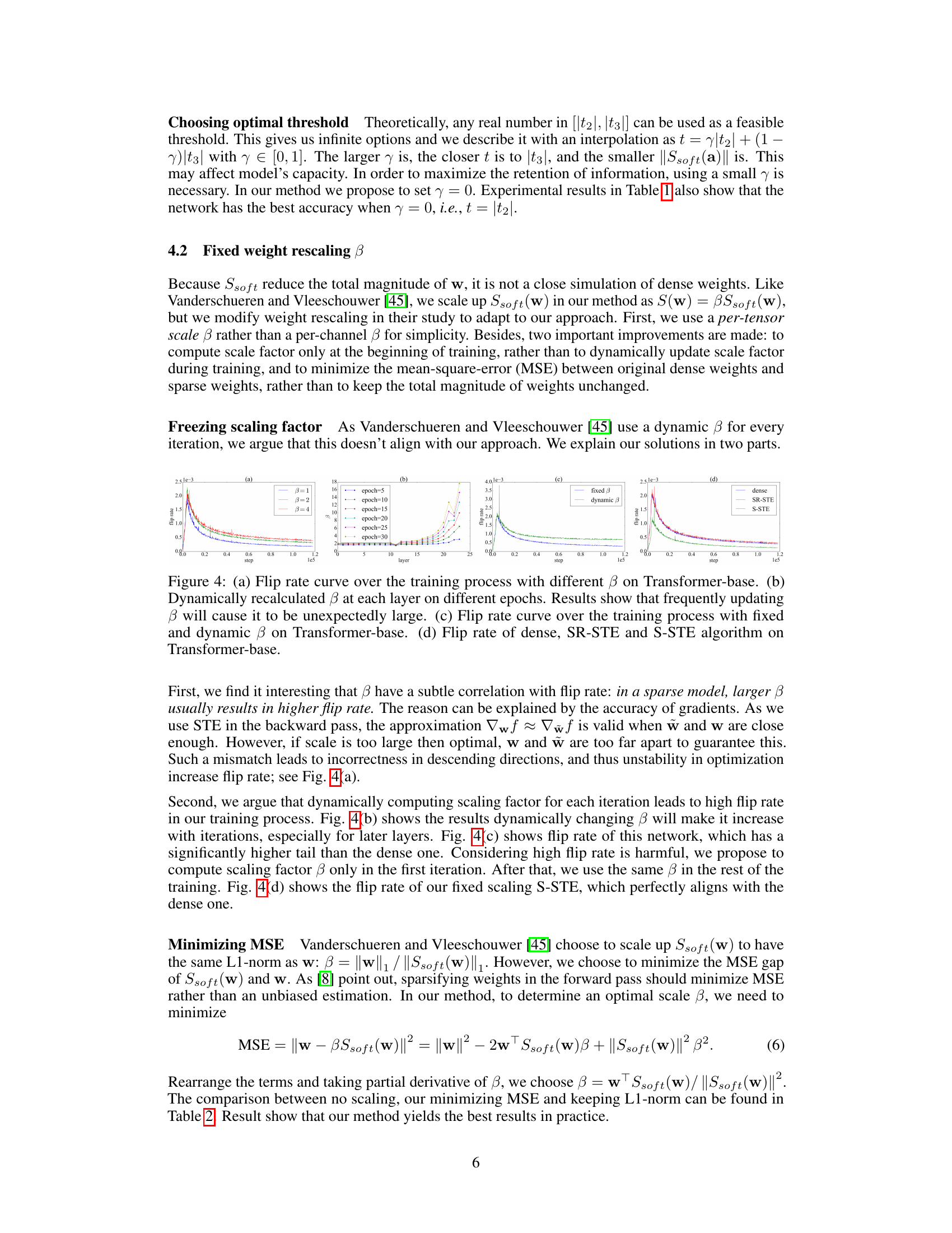
🔼 This figure visualizes the impact of different beta (β) values and updating strategies on the flip rate during the training process. Subfigure (a) shows how different constant β values affect the flip rate’s trajectory. Subfigure (b) demonstrates the effect of dynamically recalculating β at each layer throughout various epochs, revealing that frequent updates lead to unexpectedly high β values. Subfigure (c) compares the flip rate when using a fixed β versus a dynamic β, highlighting the stability benefits of a fixed β. Finally, subfigure (d) provides a direct comparison of the flip rate for dense models, models trained using SR-STE, and models trained using the proposed S-STE method.
read the caption
Figure 4: (a) Flip rate curve over the training process with different β on Transformer-base. (b) Dynamically recalculated β at each layer on different epochs. Results show that frequently updating β will cause it to be unexpectedly large. (c) Flip rate curve over the training process with fixed and dynamic β on Transformer-base. (d) Flip rate of dense, SR-STE and S-STE algorithm on Transformer-base.
More on tables

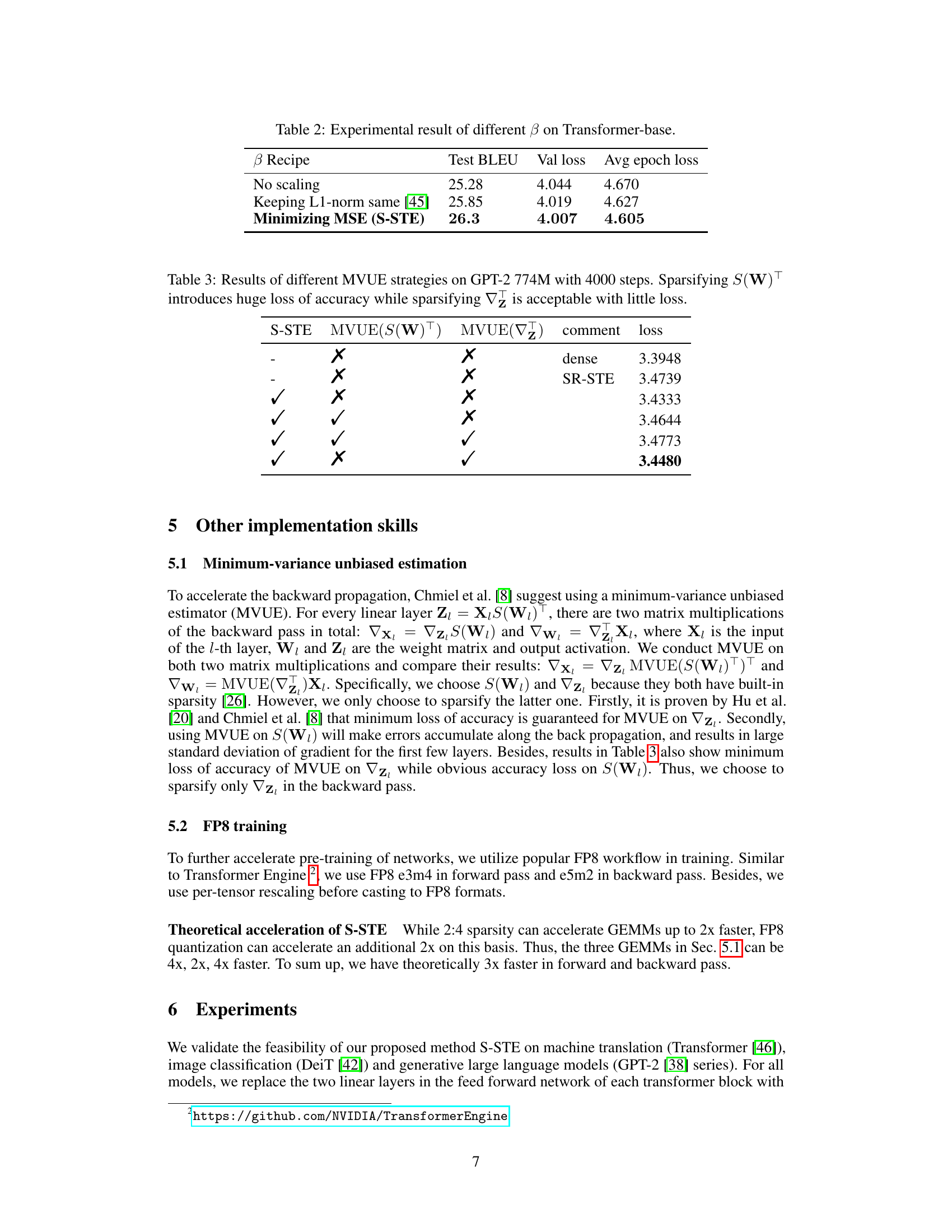
🔼 This table presents the experimental results of different beta (β) values on the Transformer-base model. It compares three different β recipes: no scaling, keeping L1-norm same, and minimizing MSE. The results show the Test BLEU score, validation loss, and average epoch loss for each β recipe. The minimizing MSE recipe (S-STE) is shown to yield the best results.
read the caption
Table 2: Experimental result of different β on Transformer-base.
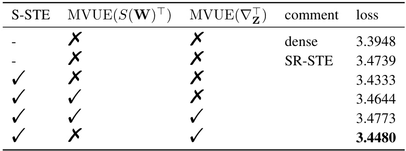
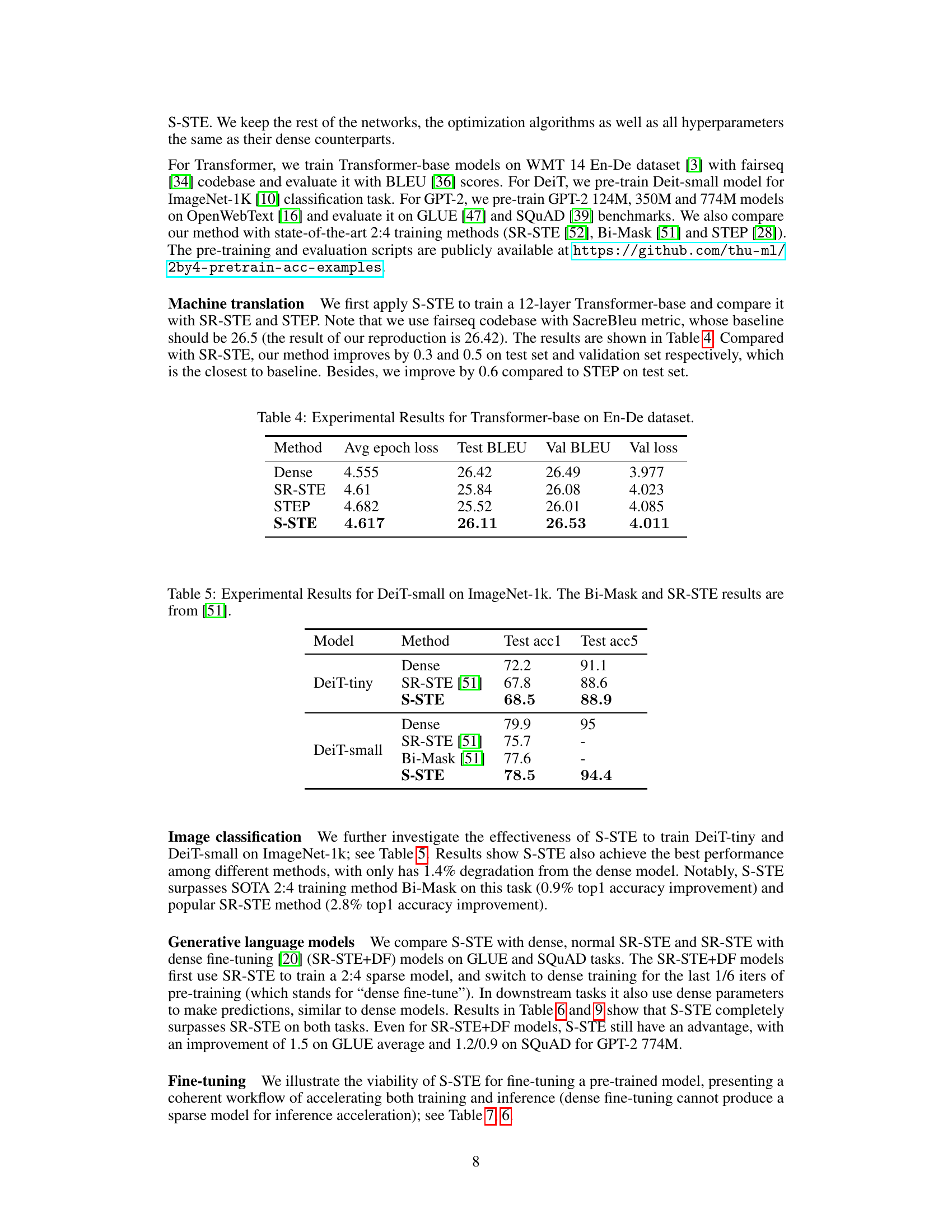
🔼 This table compares different strategies for using Minimum-Variance Unbiased Estimation (MVUE) during the training of a GPT-2 774M model with 2:4 sparsity. It shows the impact on training loss when MVUE is applied to either the sparse weight matrix S(W) or the gradient ∇z. The results indicate that applying MVUE to the gradient significantly outperforms applying it to the sparse weight matrix.
read the caption
Table 3: Results of different MVUE strategies on GPT-2 774M with 4000 steps. Sparsifying S(W) introduces huge loss of accuracy while sparsifying ∇z is acceptable with little loss.

🔼 This table presents the experimental results of training a Transformer-base model on the En-De dataset for machine translation. It compares the performance of four different methods: Dense (full-parameter model), SR-STE, STEP, and the proposed S-STE method. The metrics used for evaluation are average epoch loss, Test BLEU score, Val BLEU score, and validation loss. The results show that S-STE outperforms SR-STE and STEP, achieving BLEU scores closer to the Dense model baseline.
read the caption
Table 4: Experimental Results for Transformer-base on En-De dataset.
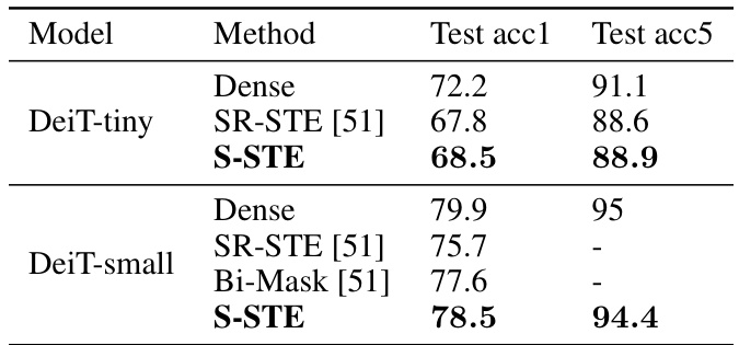
🔼 This table presents the results of image classification experiments using the DeiT-small model on the ImageNet-1k dataset. It compares the test accuracy (top-1 and top-5) achieved by three different methods: a dense model (full-weight model), SR-STE (Sparse-Regularized Straight-Through Estimator), and the proposed S-STE method. The results show the relative performance of S-STE compared to existing sparse training techniques.
read the caption
Table 5: Experimental Results for DeiT-small on ImageNet-1k. The Bi-Mask and SR-STE results are from [51].
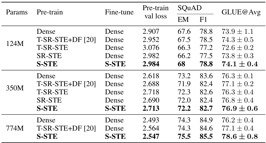
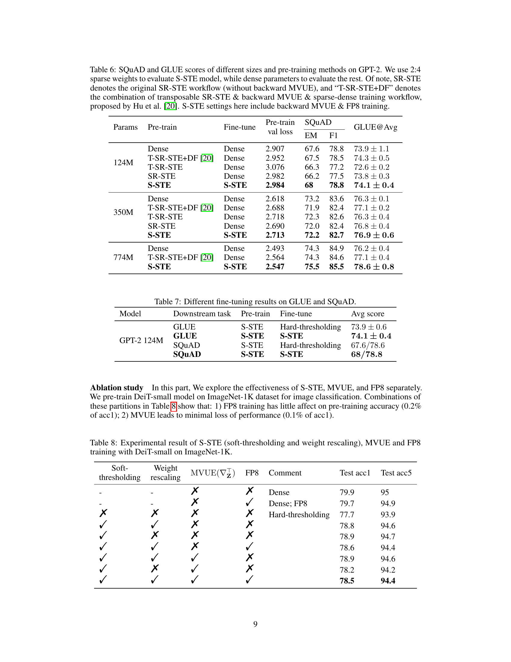
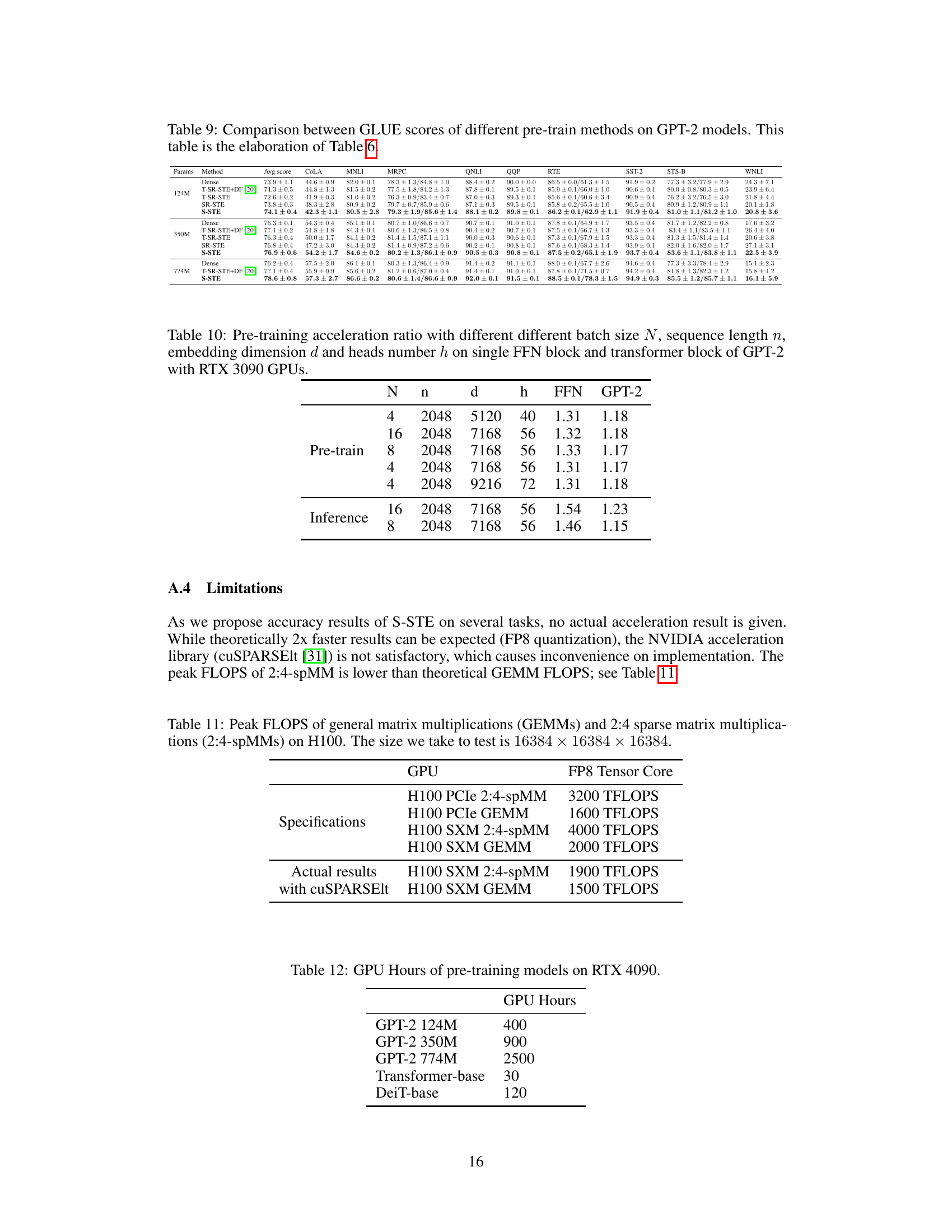
🔼 This table compares the performance of different pre-training methods (Dense, T-SR-STE+DF, T-SR-STE, SR-STE, and S-STE) on GPT-2 models of various sizes (124M, 350M, and 774M). The evaluation metrics are SQUAD (Exact Match and F1 score) and GLUE (average score). S-STE uses 2:4 sparse weights, while the other methods use dense weights for evaluation. Note that ‘T-SR-STE+DF’ represents a combination of transposable SR-STE, backward MVUE, and sparse-dense training workflow. The S-STE results use backward MVUE and FP8 training.
read the caption
Table 6: SQUAD and GLUE scores of different sizes and pre-training methods on GPT-2. We use 2:4 sparse weights to evaluate S-STE model, while dense parameters to evaluate the rest. Of note, SR-STE denotes the original SR-STE workflow (without backward MVUE), and “T-SR-STE+DF

🔼 This table shows the results of fine-tuning on the GLUE and SQUAD benchmarks using different pre-training and fine-tuning methods. The pre-training methods are S-STE (smooth straight-through estimator) and hard-thresholding. The fine-tuning methods are S-STE and hard-thresholding. The average score is reported for each combination of pre-training and fine-tuning methods.
read the caption
Table 7: Different fine-tuning results on GLUE and SQUAD.
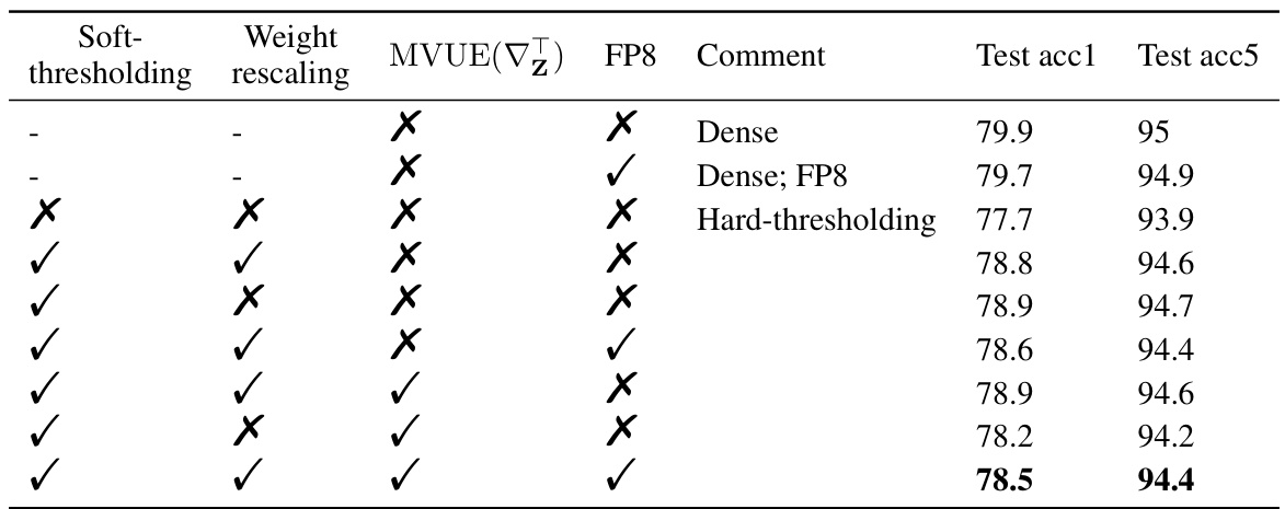
🔼 This table presents the ablation study results for the DeiT-small model trained on the ImageNet-1K dataset. It shows the impact of different components of the proposed S-STE method (soft-thresholding, weight rescaling, MVUE, and FP8 training) on the model’s performance (measured by top-1 and top-5 accuracy). Each row represents a different combination of these components, allowing researchers to evaluate their individual and combined effects on the model’s accuracy. The results highlight the contribution of each component to the overall performance of the model.
read the caption
Table 8: Experimental result of S-STE (soft-thresholding and weight rescaling), MVUE and FP8 training with DeiT-small on ImageNet-1K.

🔼 This table compares the performance of different pre-training methods (dense, T-SR-STE+DF, T-SR-STE, SR-STE, and S-STE) on GPT-2 models of varying sizes (124M, 350M, and 774M). The evaluation is done using both sparse (2:4) and dense weights. The results are presented in terms of GLUE and SQUAD scores, providing a comprehensive assessment of the various methods’ effectiveness. It highlights the impact of different components (backward MVUE, FP8 training) on S-STE’s performance.
read the caption
Table 6: SQUAD and GLUE scores of different sizes and pre-training methods on GPT-2. We use 2:4 sparse weights to evaluate S-STE model, while dense parameters to evaluate the rest. Of note, SR-STE denotes the original SR-STE workflow (without backward MVUE), and “T-SR-STE+DF” denotes the combination of transposable SR-STE & backward MVUE & sparse-dense training workflow, proposed by Hu et al. [20]. S-STE settings here include backward MVUE & FP8 training.
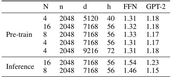
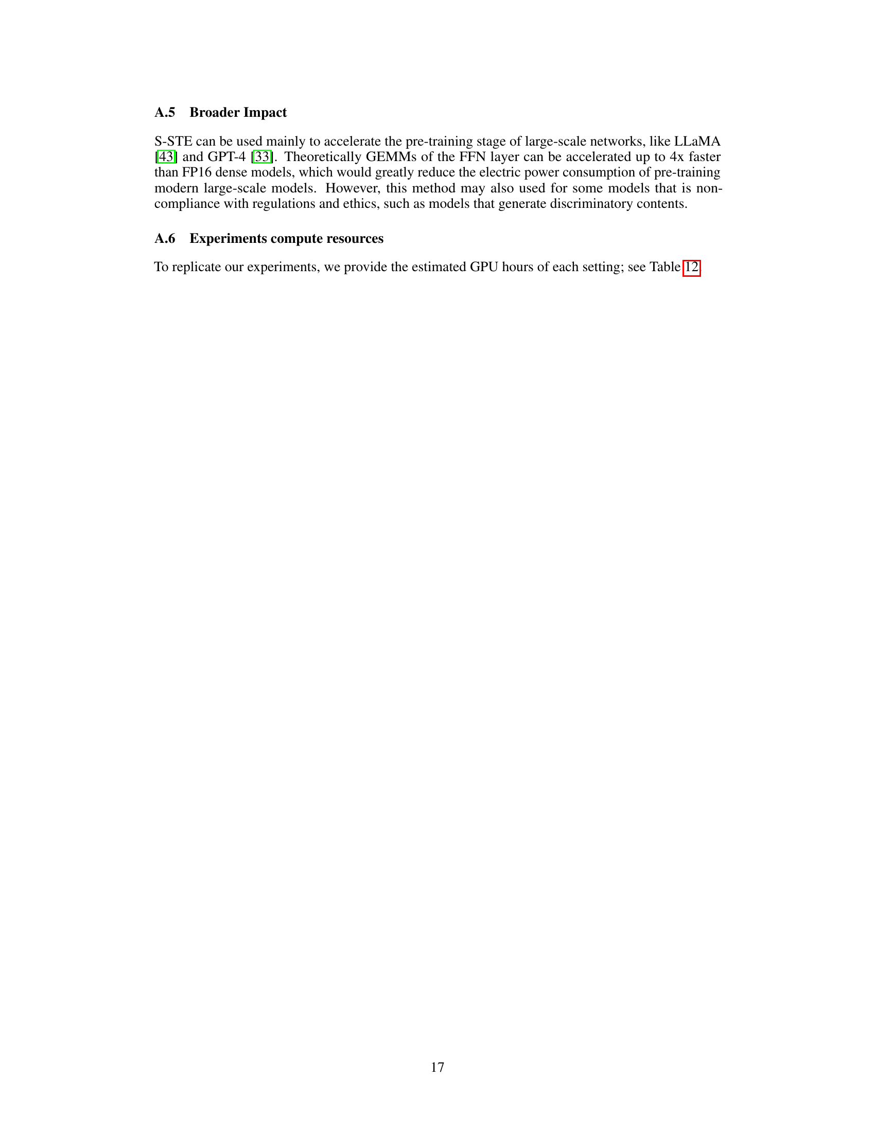
🔼 This table shows the pre-training and inference acceleration ratios achieved by the proposed S-STE method on a GPT-2 model using RTX 3090 GPUs. It demonstrates the impact of varying batch size (N), sequence length (n), embedding dimension (d), and number of heads (h) on the acceleration ratios for both the Feed-Forward Network (FFN) layer and the overall GPT-2 transformer block. The results indicate speedups achieved by S-STE in pre-training and inference scenarios.
read the caption
Table 10: Pre-training acceleration ratio with different different batch size N, sequence length n, embedding dimension d and heads number h on single FFN block and transformer block of GPT-2 with RTX 3090 GPUs.
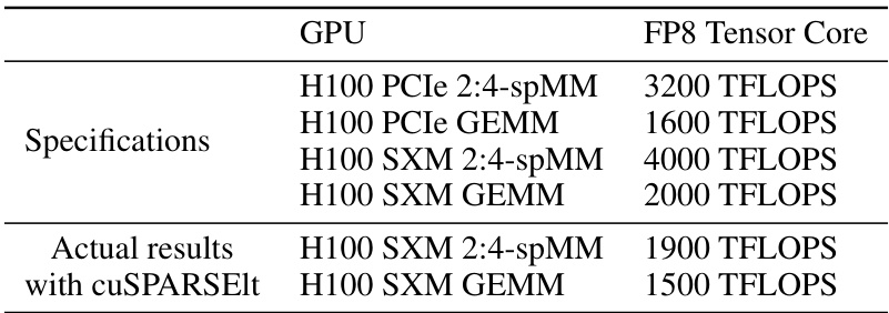
🔼 This table shows the peak FLOPS (floating point operations per second) for general matrix multiplication (GEMM) and 2:4 sparse matrix multiplication (2:4-spMM) on two different versions of the NVIDIA H100 GPU (PCIe and SXM). It highlights the difference between theoretical peak performance and the actual performance achieved using the cuSPARSElt library, demonstrating the limitations in achieving the full theoretical speedup for sparse matrix operations.
read the caption
Table 11: Peak FLOPS of general matrix multiplications (GEMMs) and 2:4 sparse matrix multiplications (2:4-spMMs) on H100. The size we take to test is 16384 × 16384 × 16384.
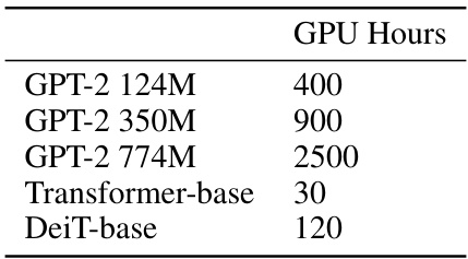
🔼 This table presents the estimated GPU hours required for pre-training different models on RTX 4090 GPUs. The models include various sizes of GPT-2 (124M, 350M, and 774M parameters), Transformer-base, and DeiT-base. These estimates are useful for researchers who want to reproduce the experiments in the paper or assess the computational resources needed for similar pre-training tasks.
read the caption
Table 12: GPU Hours of pre-training models on RTX 4090.
Full paper#
