TL;DR#
Graph Neural Networks (GNNs) often struggle with classifying non-isomorphic graphs due to limitations in their expressive power, particularly for tasks like substructure identification. Adding random noise to node features (node individualization) is a common solution, but its impact on generalization is unclear. This raises concerns about sample complexity - how much training data is needed for reliable results.
This paper theoretically analyzes the sample complexity of GNNs using node individualization, finding that permutation-equivariant methods are superior. They propose new individualization schemes based on these findings, and develop a novel GNN architecture (EGONN) specifically designed for substructure identification. Their experiments support the theoretical analysis, showcasing the effectiveness of the proposed techniques on both synthetic and real-world datasets. This work significantly contributes to our understanding of GNN expressiveness and generalization, offering valuable insights for improving GNN design and application.
Key Takeaways#
Why does it matter?#
This paper is crucial for researchers working with graph neural networks (GNNs). It addresses the critical issue of GNN expressivity limitations and proposes novel solutions to enhance their generalization capabilities. The theoretical analysis of sample complexity and the introduction of novel individualization schemes are valuable contributions that will likely inspire further research in GNN design and optimization, particularly for tasks like substructure identification.
Visual Insights#
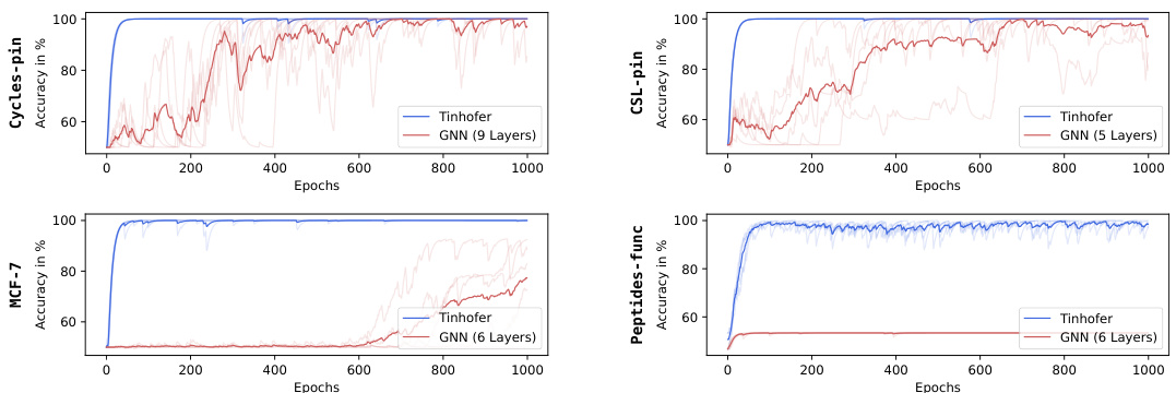
🔼 The figure shows the accuracy for two different models over 1000 epochs for four different datasets (two synthetic and two real-world). The first model is a standard GNN with multiple layers (the number of layers is specified for each dataset), while the second model is a 1-layer GNN that utilizes the Tinhofer individualization scheme. The results demonstrate that the GNN with Tinhofer individualization converges faster and more stably, particularly for real-world datasets, where the standard GNN struggles to reach high accuracy within the tested 1000 epochs. This highlights the benefit of node individualization in improving the expressivity of shallow GNNs.
read the caption
Figure 2: Accuracy for GNNK and GNN10 Tinhofer over 1000 epochs on synthetic datasets Cycles-pin and CSL-pin and real-world datasets MCF-7 [63, 37] and Peptites-func [55, 17].

🔼 This table presents the training and test accuracies for substructure identification on 3-regular graphs using different methods. The methods include standard GNNs with different node individualization schemes (none, relational pooling (RP), and Tinhofer) and a novel architecture called EGONN with varying individualization schemes. The goal is to assess the performance of these methods in detecting the presence of specific subgraphs (3-cycle, 4-cycle, 5-cycle, and complete bipartite graph K2,3) within the larger graphs.
read the caption
Table 1: Train and test accuracies for the substructure identification task on 3-regular graphs.
In-depth insights#
GNN Expressivity#
The expressivity of Graph Neural Networks (GNNs) is a central theme in the paper, focusing on their inherent limitations. GNNs are constrained by the Weisfeiler-Leman (WL) test, which limits their ability to distinguish non-isomorphic graphs. The paper explores how node individualization schemes, which introduce unique identifiers to nodes, overcome this limitation by breaking graph symmetries, enabling GNNs to reach universal expressivity as function approximators. However, this increased expressivity comes with trade-offs, impacting sample complexity. The research delves into understanding this trade-off. Various node individualization techniques are compared, highlighting the importance of permutation-equivariance to minimize sample complexity. Ultimately, the paper provides a theoretical analysis and empirical validation of how different individualization schemes impact GNN expressivity and generalization, paving the way for more effective GNN architectures.
Sample Complexity#
The concept of sample complexity, crucial in machine learning, is thoroughly investigated in this research paper. It focuses on graph neural networks (GNNs) and their ability to generalize from limited training data. The authors explore the impact of node individualization schemes on sample complexity, demonstrating that permutation-equivariant methods lead to lower complexity. VC dimension and covering number bounds are employed for a theoretical analysis, providing a framework to design GNN architectures with improved generalization capabilities. The study highlights a key trade-off between expressivity and sample complexity, showing that achieving universal expressiveness through node individualization can come at the cost of increased sample requirements. Novel individualization schemes are proposed, aiming for a balance between enhanced expressivity and manageable sample complexity. The theoretical findings are further validated through experiments on synthetic and real-world datasets, confirming the practical implications of the theoretical analysis. The work contributes significantly to understanding and improving the generalization performance of GNNs, particularly in scenarios with limited data.
Node Individualization#
Node individualization techniques are crucial for enhancing the expressive power of Graph Neural Networks (GNNs). By breaking graph symmetries, these methods allow GNNs to learn more complex and nuanced representations, surpassing the limitations imposed by the Weisfeiler-Lehman test. Random Node Initialization (RNI) and Relational Pooling (RP) are prominent examples, each with its own advantages and trade-offs. While RNI introduces randomness, RP leverages node labels for partitioning, creating unique identifiers. The choice of method significantly affects the sample complexity, as permutation-equivariant techniques, such as a refined individualization scheme based on the Tinhofer algorithm, demonstrate superior generalization capabilities due to their lower VC dimension. This trade-off between expressivity and sample complexity is a central theme, highlighting the importance of designing individualization schemes that balance model capacity and generalization performance. The theoretical analysis, employing VC-dimension and covering number bounds, provides valuable insights into the impact of different approaches on learning efficiency, suggesting that careful selection of an individualization method is critical for successful GNN applications.
Substructure ID#
The section on substructure identification delves into a crucial challenge in graph neural networks (GNNs): detecting the presence of specific subgraph patterns within larger graphs. The authors demonstrate that standard message-passing GNNs are inherently limited in this task, highlighting the need for enhanced expressiveness. They propose a novel architecture, EGONN, which cleverly leverages node individualization techniques on subgraphs (ego-nets) to overcome the limitations of traditional methods. This approach is theoretically grounded, providing VC-dimension bounds that demonstrate the improved generalization capabilities of EGONN compared to other methods. The experimental results on challenging datasets validate the theoretical claims, showcasing EGONN’s superior performance in identifying substructures while managing model complexity effectively. A key takeaway is that smartly applying node individualization to smaller, manageable subgraphs, rather than the entire graph, offers a practical way to boost GNNs’ power for substructure identification, while mitigating issues like overfitting and under-reaching often associated with deeper GNN architectures.
Future Directions#
Future research should prioritize developing tighter theoretical bounds for GNNs by addressing the limitations of current approaches like VC dimension and Rademacher complexity. Investigating data augmentation techniques for individualization schemes, especially their impact on generalization, is crucial. Developing novel architectures that balance expressivity and computational complexity is also essential, as is exploring alternative metrics that better capture the properties of graph data and GNN model behavior. The theoretical analysis should be extended to cover a wider range of individualization schemes and graph datasets to enhance the generality of the findings. Finally, a focus on practical applications and empirical validations will solidify the theoretical contributions, potentially leading to improvements in tasks like substructure identification and graph classification.
More visual insights#
More on figures
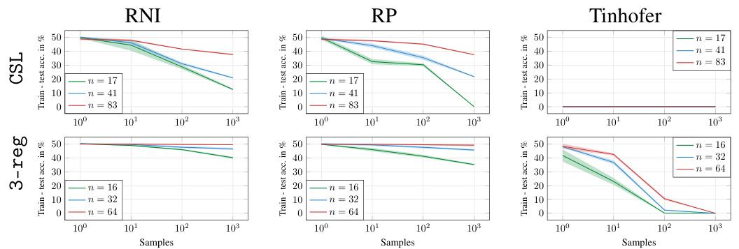
🔼 This figure displays the difference between training and testing accuracy for Graph Neural Networks (GNNs) using three different node individualization schemes (RNI, RP, and Tinhofer). The results are shown for two types of graphs: CSL graphs (circular skip link) and 3-regular graphs. Different sizes of graphs are tested (n = 16, 17, 32, 41, 64, 83). The x-axis represents the number of samples used in training, while the y-axis represents the difference between training and test accuracy. The figure helps to illustrate how the sample complexity varies depending on the individualization scheme and graph structure.
read the caption
Figure 3: Difference between test and training accuracy for GNNs with the RNI, RP and Tinhofer individualization schemes, on datasets of CSL and 3-regular graphs of various sizes.
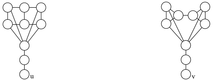
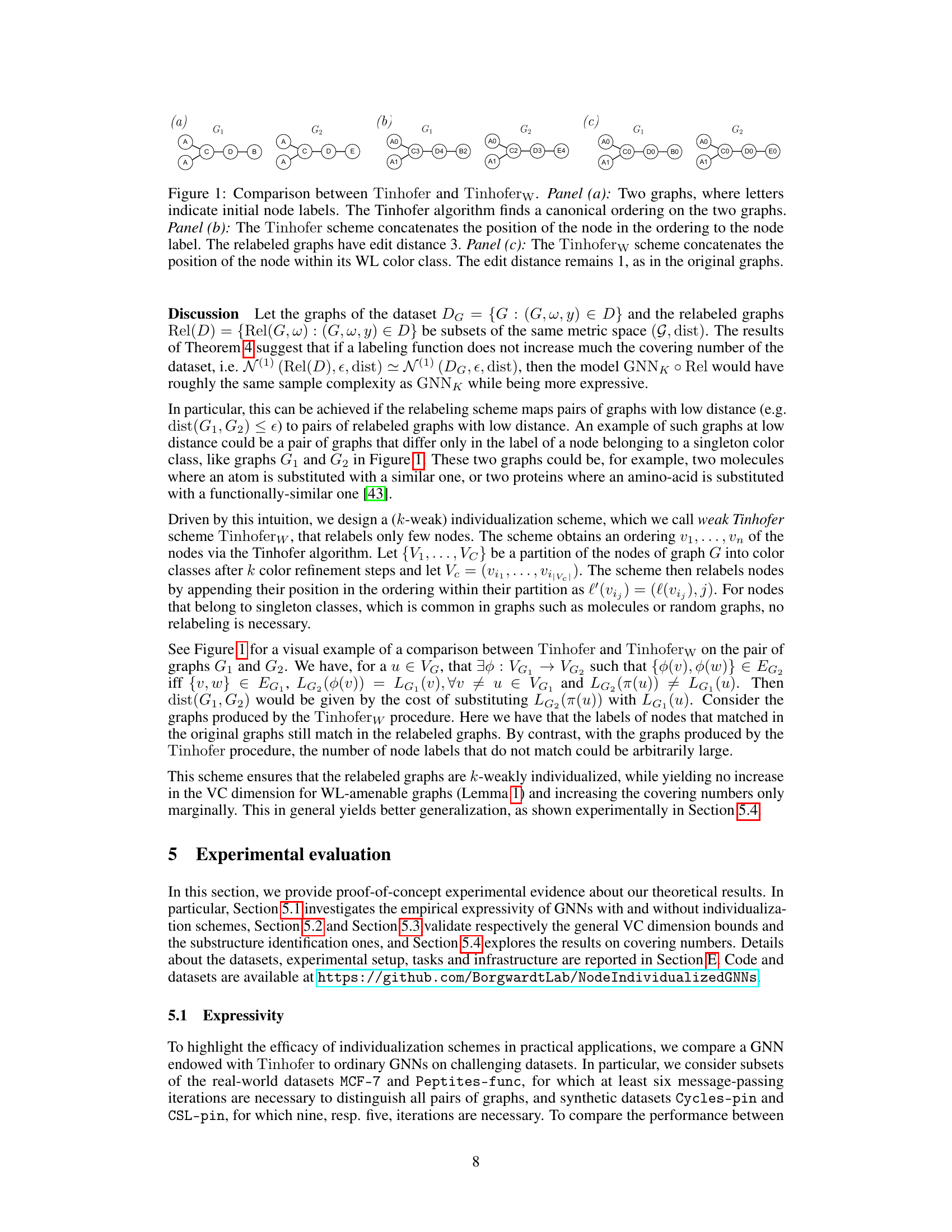
🔼 This figure compares the Tinhofer and the improved Tinhoferw node individualization schemes. It shows how the Tinhofer scheme, by concatenating node position in a canonical ordering to node labels, can significantly increase the edit distance between similar graphs, making them harder to distinguish with a GNN. Conversely, the Tinhoferw scheme, by only concatenating the position within the Weisfeiler-Lehman color class, preserves the edit distance, illustrating its superior ability to maintain graph similarity while achieving individualization.
read the caption
Figure 1: Comparison between Tinhofer and Tinhoferw. Panel (a): Two graphs, where letters indicate initial node labels. The Tinhofer algorithm finds a canonical ordering on the two graphs. Panel (b): The Tinhofer scheme concatenates the position of the node in the ordering to the node label. The relabeled graphs have edit distance 3. Panel (c): The Tinhoferw scheme concatenates the position of the node within its WL color class. The edit distance remains 1, as in the original graphs.

🔼 This figure shows the covering numbers for the NCI dataset using different node individualization schemes. The x-axis represents the log10 of epsilon (ε), and the y-axis represents the covering number. The curves show how the number of balls of radius ε needed to cover the space of functions (represented by different individualization schemes) changes with ε. The comparison provides insights into the sample complexity of graph neural networks using different node individualization schemes.
read the caption
Figure 5: Covering numbers for the NCI dataset
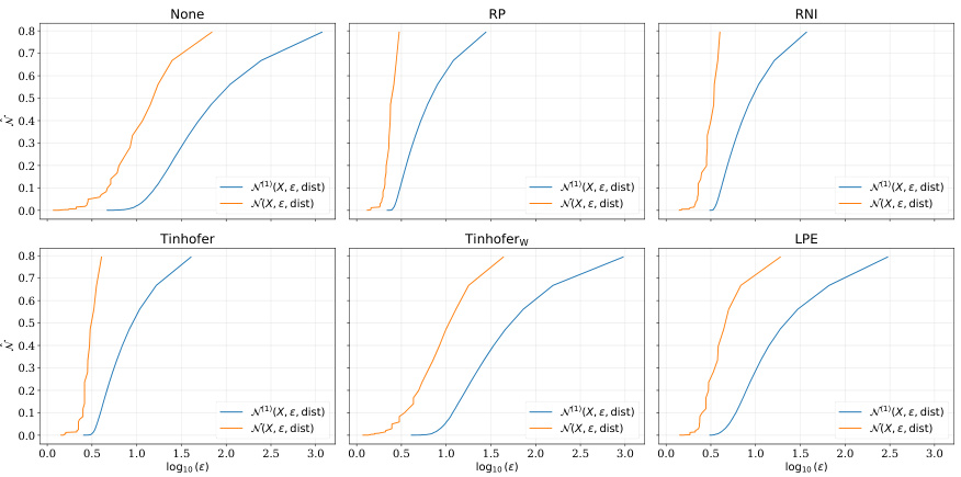
🔼 This figure shows the covering numbers for the NCI dataset using different node individualization schemes. The x-axis represents the logarithm of epsilon (ε), which is a parameter related to the accuracy of the covering. The y-axis represents the covering number, which is a measure of the complexity of the function class. Each subplot corresponds to a different individualization scheme: None, RP, RNI, Tinhofer, Tinhoferw, and LPE. The blue and orange lines represent the covering number for the 1-norm and ∞-norm, respectively. The figure shows that the covering numbers for the Tinhofer and Tinhoferw schemes are significantly lower than those for the other schemes, suggesting that these schemes lead to simpler function classes and potentially better generalization performance.
read the caption
Figure 5: Covering numbers for the NCI dataset
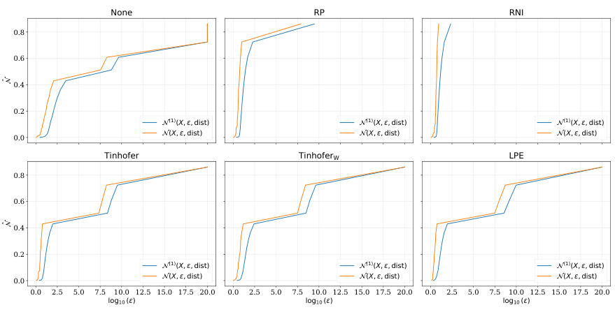
🔼 This figure shows the covering numbers for the NCI dataset using different node individualization schemes. The x-axis represents the log10 of epsilon (ε), which is a parameter used in calculating covering numbers. The y-axis shows the covering number, indicating the minimum number of balls of radius ε needed to cover the set of graphs. The different lines represent different node individualization schemes: None, RP, RNI, Tinhofer, Tinhoferw, and LPE. The plot compares the 1-norm and ∞-norm covering numbers for each scheme, offering insights into the sample complexity of graph neural networks (GNNs) under various individualization strategies.
read the caption
Figure 5: Covering numbers for the NCI dataset

🔼 This figure displays the difference between training and testing accuracy for GNNs using three different individualization schemes (RNI, RP, and Tinhofer) on two types of graphs: CSL (circular skip link) graphs and 3-regular graphs. Each type of graph is tested at various sizes (indicated by ’n’ representing the number of nodes). The plots show how the generalization gap (difference between train and test accuracy) changes as the amount of training data increases, for each individualization method and graph type. The goal is to show how different individualization schemes impact the generalization capability of GNNs. The finding is that Tinhofer tends to exhibit smaller generalization gaps, particularly for the CSL graphs, showing its greater efficiency and effectiveness.
read the caption
Figure 3: Difference between test and training accuracy for GNNs with the RNI, RP and Tinhofer individualization schemes, on datasets of CSL and 3-regular graphs of various sizes.
More on tables

🔼 This table presents a comparison of the performance of different GNN models (with and without individualization schemes) on four real-world datasets: NCI1, Mutagenicity, IMDB-b, and COLLAB-b. For each dataset and model, it shows the covering number (N), the test accuracy (Test), and the difference between test and train accuracy (Diff). The covering number serves as a proxy for sample complexity. The results illustrate the impact of different node individualization schemes on generalization performance.
read the caption
Table 2: Covering numbers and classification accuracies on real-world datasets.

🔼 This table presents information on eleven graph datasets used in the paper’s experiments. For each dataset, it lists the number of graphs, the number of classes, the average number of nodes and edges per graph, whether the graphs have node labels (+ indicates presence, - indicates absence), and the minimum number of Weisfeiler-Lehman (WL) iterations needed to distinguish all graphs in the dataset. A ‘-’ indicates that WL iterations cannot distinguish all graphs in the dataset.
read the caption
Table 3: Overview of real-world and synthetic graph dataset properties. Datasets marked (*) are composed of subsets of the original datasets. The column “WL number” denotes the minimum number of WL iterations necessary to distinguish all graphs. The entry (-) in this column indicates that this number does not exist, i.e., not all graphs can be distinguished by color refinement.
Full paper#
