TL;DR#
Many machine learning models optimize risk functions based on empirical data distributions, potentially leading to poor out-of-sample performance due to distributional uncertainty. Distributionally Robust Optimization (DRO) offers solutions, but existing approaches often lack favorable statistical guarantees or practical tractability. This is a significant limitation, especially when dealing with small sample sizes and complex data generating processes.
This paper introduces a novel robust optimization criterion that addresses these shortcomings. It leverages Bayesian Nonparametrics (specifically, Dirichlet processes) to model distributional uncertainty and incorporates smooth ambiguity aversion to manage uncertainty-averse preferences. The approach yields favorable finite-sample and asymptotic performance guarantees, with connections to standard regularized techniques like Ridge and Lasso regressions. The authors propose tractable approximations, demonstrating the criterion’s practical applicability through simulated and real datasets. The method naturally lends itself to standard gradient-based numerical optimization.
Key Takeaways#
Why does it matter?#
This paper is crucial for researchers grappling with distributional uncertainty in machine learning and statistics. It offers a novel robust optimization criterion combining Bayesian nonparametrics and smooth ambiguity aversion, providing strong theoretical guarantees and practical advantages. The proposed method enhances out-of-sample performance, offering new avenues for developing robust and reliable machine learning models.
Visual Insights#

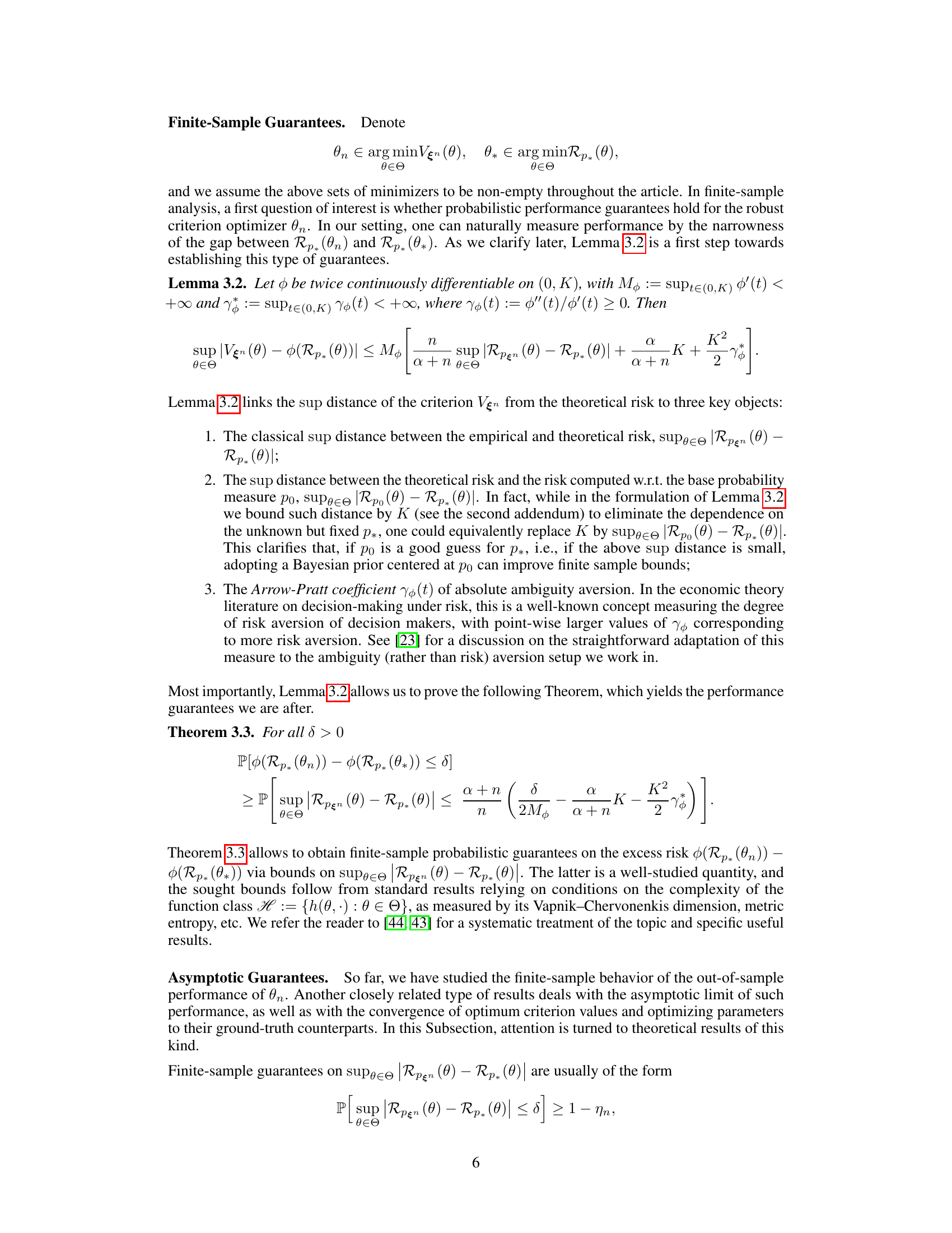
🔼 This figure illustrates the concept of smooth ambiguity aversion. Two decisions, θ₁ and θ₂, have the same expected risk (R*) under a distribution Q, but θ₁ has less variability in its risk across different possible models (p₁ and p₂). A convex function φ applied to the expected risks highlights that the ambiguity-averse criterion prefers θ₁ due to its lower risk variability.
read the caption
Figure 1: Graphical display of smooth ambiguity aversion at work. Although θ₁ and θ₂ yield the same loss R* in Q-expectation, the ambiguity averse criterion favors the less variable decision θ₁. Graphically, this is because the orange line connecting φ(Rp₁(θ₁)) to φ(Rp₂(θ₁)) lies (point-wise) below the line connecting φ(Rp₁(θ₂)) to φ(Rp₂(θ₂)).

🔼 This table compares the performance of three methods for binary classification on the Pima Indian Diabetes dataset: unregularized logistic regression, L1-regularized logistic regression, and the proposed distributionally robust method. The metrics reported are the average out-of-sample loss and the standard deviation of the out-of-sample loss across multiple runs.
read the caption
Table 1. Comparison of average and standard deviation of the out-of-sample performance (out-of-sample expected logistic loss) of the three employed methods for binary classification on the Pima Indian Diabetes dataset.
In-depth insights#
Robust Risk Minimization#
Robust risk minimization seeks to mitigate the impact of uncertainty in risk estimation, a critical challenge in machine learning and statistics. Standard empirical risk minimization can be overly sensitive to noise and outliers, leading to poor generalization. Robust methods aim to improve model stability and out-of-sample performance by considering a range of plausible data distributions or by reducing the influence of extreme data points. Bayesian nonparametrics offers a powerful framework for addressing this challenge. Instead of assuming a fixed data distribution, these methods allow for flexible modeling of uncertainty, creating a more robust risk estimate. Regularization techniques play an important role, often providing an implicit form of robustness by constraining model complexity and reducing overfitting. The choice of loss function, regularization method, and prior distribution significantly influence the robustness properties of the resulting risk minimization procedure. The integration of Bayesian methods with robust optimization techniques represents a promising direction for improving the reliability and generalizability of machine learning models in the presence of uncertainty.
Bayesian Nonparametrics#
Bayesian nonparametrics offers a powerful approach to statistical modeling by relaxing the restrictive assumption of fixed, finite-dimensional parameter spaces. Instead of specifying a parametric model a priori, Bayesian nonparametrics employs flexible, infinite-dimensional distributions to represent the uncertainty in the data-generating process. This approach allows the model to adapt its complexity to the data, avoiding the potential pitfalls of misspecification inherent in parametric methods. A key advantage is the ability to incorporate prior knowledge through appropriate base measures, while simultaneously allowing the data to shape the posterior distribution. Popular examples include Dirichlet processes and Gaussian processes, which offer tractable computational methods for inference. The inherent flexibility of Bayesian nonparametrics makes it particularly well-suited for applications where the data-generating process is complex and unknown, such as in machine learning, density estimation, and clustering. However, challenges in computational complexity and theoretical guarantees remain areas of active research.
Smooth Ambiguity#
The concept of “Smooth Ambiguity” in decision theory offers a nuanced approach to modeling how individuals make choices under uncertainty. Unlike traditional expected utility theory, which assumes a single, precisely known probability distribution, smooth ambiguity acknowledges the inherent ambiguity or uncertainty surrounding the true distribution. This ambiguity isn’t treated as a worst-case scenario (as in some robust optimization methods) but is instead integrated into the decision-making process using a smoothing function. This smoothing function, often a convex function, reflects the decision-maker’s aversion to ambiguity. The more convex the function, the greater the aversion and the stronger the preference for options that perform well across a range of plausible distributions, thus mitigating the impact of distributional uncertainty. This framework bridges the gap between purely objective Bayesian models (where expectations are taken over the posterior distribution) and purely subjective worst-case approaches. It provides a more realistic representation of decision-making under uncertainty, where preferences for robust outcomes are incorporated through a flexible functional form.
SBMC & MDMC#
The paper introduces SBMC (Stick-Breaking Monte Carlo) and MDMC (Multinomial-Dirichlet Monte Carlo) as tractable approximation methods for the distributionally robust optimization criterion. SBMC leverages the stick-breaking representation of the Dirichlet process, iteratively sampling weights and locations to approximate the posterior. MDMC utilizes a finite-dimensional Dirichlet approximation, simplifying calculations by approximating the infinite mixture with a finite number of components. Both methods address the computational challenge of directly evaluating the infinite-dimensional integral inherent in the proposed criterion. The choice between SBMC and MDMC involves a trade-off: SBMC provides a potentially more accurate approximation but is computationally more expensive. MDMC offers faster computation but may sacrifice some accuracy. The paper suggests that MDMC is generally preferable due to its well-behaved weights, making it more efficient for practical applications while maintaining sufficient accuracy. The effectiveness of both methods is empirically demonstrated through various simulation studies and real data experiments, showcasing their utility in enhancing the robustness and stability of the proposed optimization procedure.
Future Research#
The paper’s ‘Future Research’ section would ideally explore several key areas. First, extending the methodology to more complex data structures beyond iid or exchangeable data is crucial. The current method’s limitations in handling time-series or other dependent data should be addressed. Second, a deeper exploration of the method’s hyperparameter configuration and sensitivity is warranted. The influence of the prior distribution and the convexity parameter on performance needs further investigation to provide more practical guidance on model selection. Third, assessing the algorithm’s scalability and computational efficiency with larger datasets is important. While the paper demonstrates feasibility on moderate-sized datasets, its ability to handle big data and complex models needs to be evaluated. Fourth, applying the robust optimization framework to different learning paradigms and loss functions, such as deep learning tasks, will be beneficial to explore its wider applicability. Finally, a more thorough investigation into the theoretical and practical connections between the nonparametric Bayesian framework, decision theory under ambiguity, and the observed robustness should be explored, potentially revealing deeper insights into the method’s strengths and limitations.
More visual insights#
More on figures
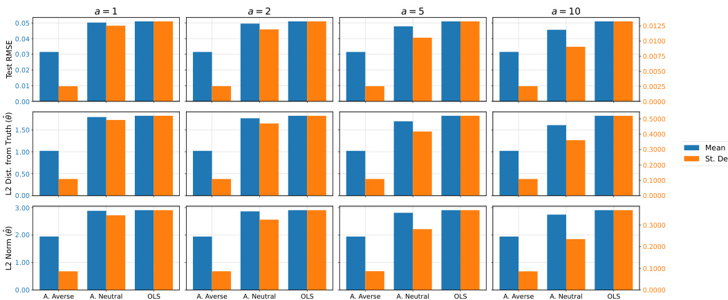
🔼 This figure displays the results of a high-dimensional sparse linear regression simulation study. Three different methods are compared: an ambiguity-averse approach (the proposed method), an ambiguity-neutral approach (regularized regression), and ordinary least squares (OLS). The performance is evaluated across four different values of the concentration parameter (a = 1, 2, 5, 10) using three metrics: test RMSE (root mean squared error), L2 distance of the estimated coefficient vector from the true vector, and the L2 norm of the estimated coefficient vector. The bars represent the mean and standard deviation of each metric across 200 simulations. The results show that the ambiguity-averse method generally outperforms the others in terms of both average performance and stability (lower standard deviation).
read the caption
Figure 2: Simulation results for the high-dimensional sparse linear regression experiment. Bars report the mean and standard deviation (across 200 sample simulations) of the test RMSE, L2 distance of estimated coefficient vector θ from the data-generating one, and the L2 norm of θ. Results are shown for the ambiguity-averse, ambiguity-neutral, and OLS procedures. Note: The left (blue) axis refers to mean values, the right (orange) axis to standard deviation values.

🔼 The figure shows the results of a simulation study comparing three different methods for estimating the mean of a Gaussian distribution in the presence of outliers. The methods are: ambiguity-averse, ambiguity-neutral, and maximum likelihood estimation (MLE). For each method, the figure displays the mean and standard deviation of the test mean negative log-likelihood and the absolute distance of the estimated parameter from the true value (0) across 100 simulations. The results demonstrate that the ambiguity-averse method outperforms the other two in terms of both average performance and variability.
read the caption
Figure 3: Simulation results from the experiment on Gaussian mean estimation with outliers. Bars report the mean and standard deviation (across 100 sample simulations) of the test mean negative log-likelihood and the absolute value distance of the estimated parameter from 0 (the data-generating value). Results are shown for the ambiguity-averse, ambiguity-neutral, and MLE procedures. Note: The left (blue) axis refers to mean values, the right (orange) axis to standard deviation values.
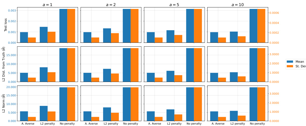
🔼 This figure displays the performance comparison among three different methods in a high-dimensional sparse logistic regression task. The methods are the proposed ambiguity-averse method, L2-regularized logistic regression, and unregularized logistic regression. The results across 200 simulations are shown for three metrics: test average loss, L2 distance from the true coefficient vector, and the L2 norm of the estimated coefficient vector. Each bar represents the mean and standard deviation of the metric across the simulations for a given method and regularization parameter (α). The figure demonstrates that the ambiguity-averse method shows improvement in terms of average performance and reduced variability, particularly for smaller α values.
read the caption
Figure 4: Simulation results for the high-dimensional sparse logistic regression experiment. Bars report the mean and standard deviation (across 200 sample simulations) of the test average loss, L2 distance of estimated coefficient vector θ from the data-generating one, and the L2 norm of θ. Results are shown for the ambiguity-averse, L2-regularized, and un-regularized procedures. Note: The left (blue) axis refers to mean values, the right (orange) axis to standard deviation values.
More on tables

🔼 This table compares the performance of three methods for binary classification on the Pima Indian Diabetes dataset: unregularized logistic regression, L1-regularized logistic regression, and the proposed distributionally robust method. The comparison focuses on the average out-of-sample loss and the standard deviation of the loss, highlighting the robustness of the proposed approach.
read the caption
Table 1: Comparison of average and standard deviation of the out-of-sample performance (out-of-sample expected logistic loss) of the three employed methods for binary classification on the Pima Indian Diabetes dataset.

🔼 This table presents the results of a linear regression experiment on the Wine Quality dataset. It compares the average and standard deviation of the out-of-sample loss for three methods: unregularized linear regression, L1-regularized linear regression (LASSO), and the distributionally robust method proposed in the paper. The distributionally robust method shows comparable average performance to LASSO with significantly lower standard deviation, indicating greater robustness.
read the caption
Table 2. Comparison of average and standard deviation of the out-of-sample performance (out-of-sample expected squared loss) of the three employed methods for linear regression on the Wine Quality dataset.

🔼 This table presents the results of a linear regression experiment on the Liver Disorders dataset. It compares the average out-of-sample loss and standard deviation across three methods: unregularized linear regression, L1-regularized linear regression, and the distributionally robust method proposed in the paper. The results demonstrate that the distributionally robust method offers both lower average error and lower variability in performance compared to the other two methods.
read the caption
Table 3: Comparison of average and standard deviation of the out-of-sample performance (out-of-sample expected squared loss) of the three employed methods for linear regression on the Liver Disorders dataset.
Full paper#

