TL;DR#
Analyzing large language models requires storing vast quantities of gradients or Hessian vector products (HVPs), creating significant memory challenges. Traditional methods struggle to scale, particularly for tasks like training data attribution (TDA), Hessian spectral analysis, and intrinsic dimension calculation. These limitations prevent deeper understanding of these complex models.
The paper introduces novel, hardware-optimized sketching algorithms (AFFD, AFJL, QK) with theoretical guarantees to efficiently address these memory bottlenecks. Experiments show that these new methods improve scalability for TDA and Hessian analysis. Furthermore, the study reveals that pre-trained language models may have much higher intrinsic dimensionality than previously thought, especially for generative tasks. The analysis of the Hessian spectra provides further insights, challenging commonly held assumptions.
Key Takeaways#
Why does it matter?#
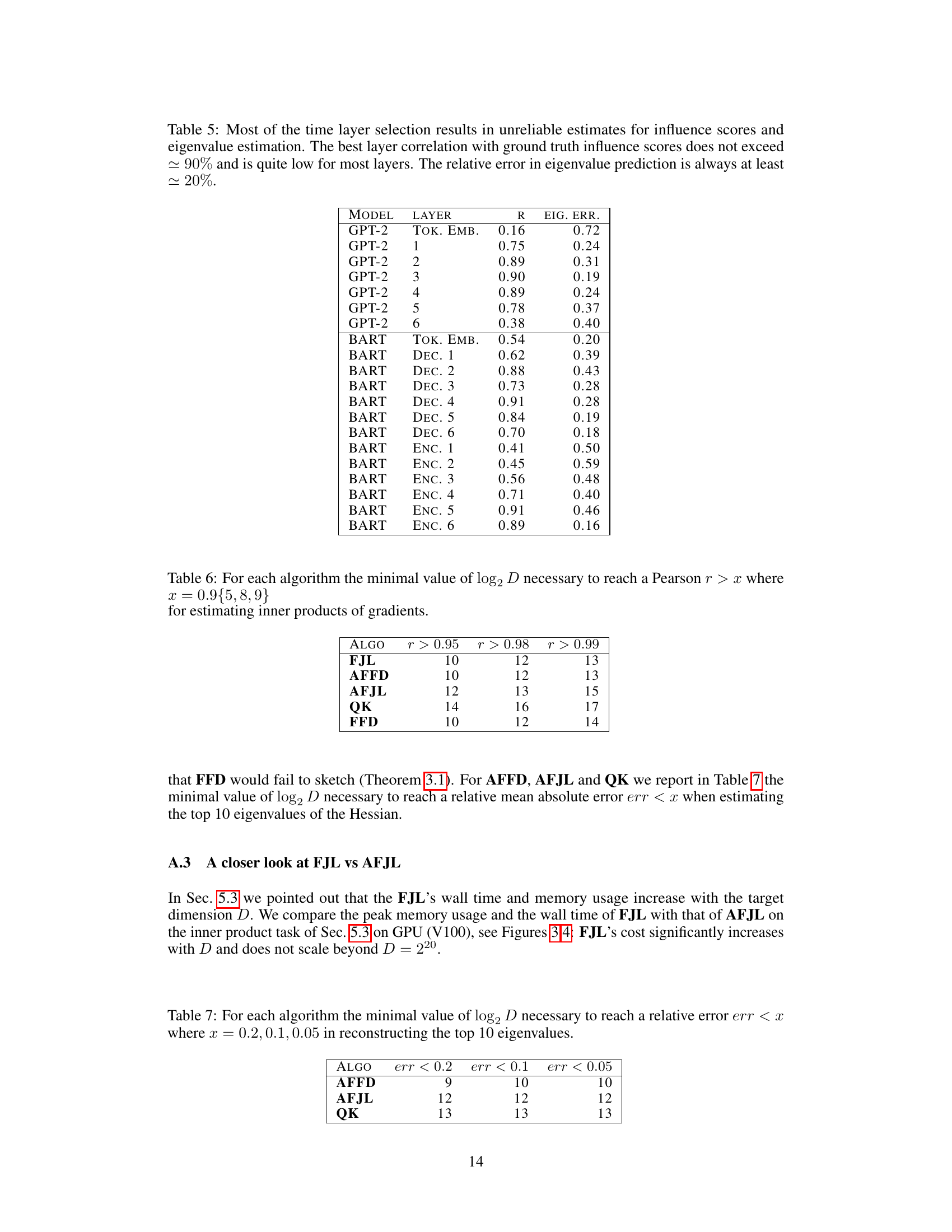
This paper is crucial for researchers working with large-scale machine learning models. It directly addresses the memory limitations hindering the analysis of gradients and Hessians, providing efficient sketching algorithms optimized for modern hardware. The new insights into the intrinsic dimensionality and Hessian properties of large language models open exciting avenues for future research in model understanding and optimization.
Visual Insights#

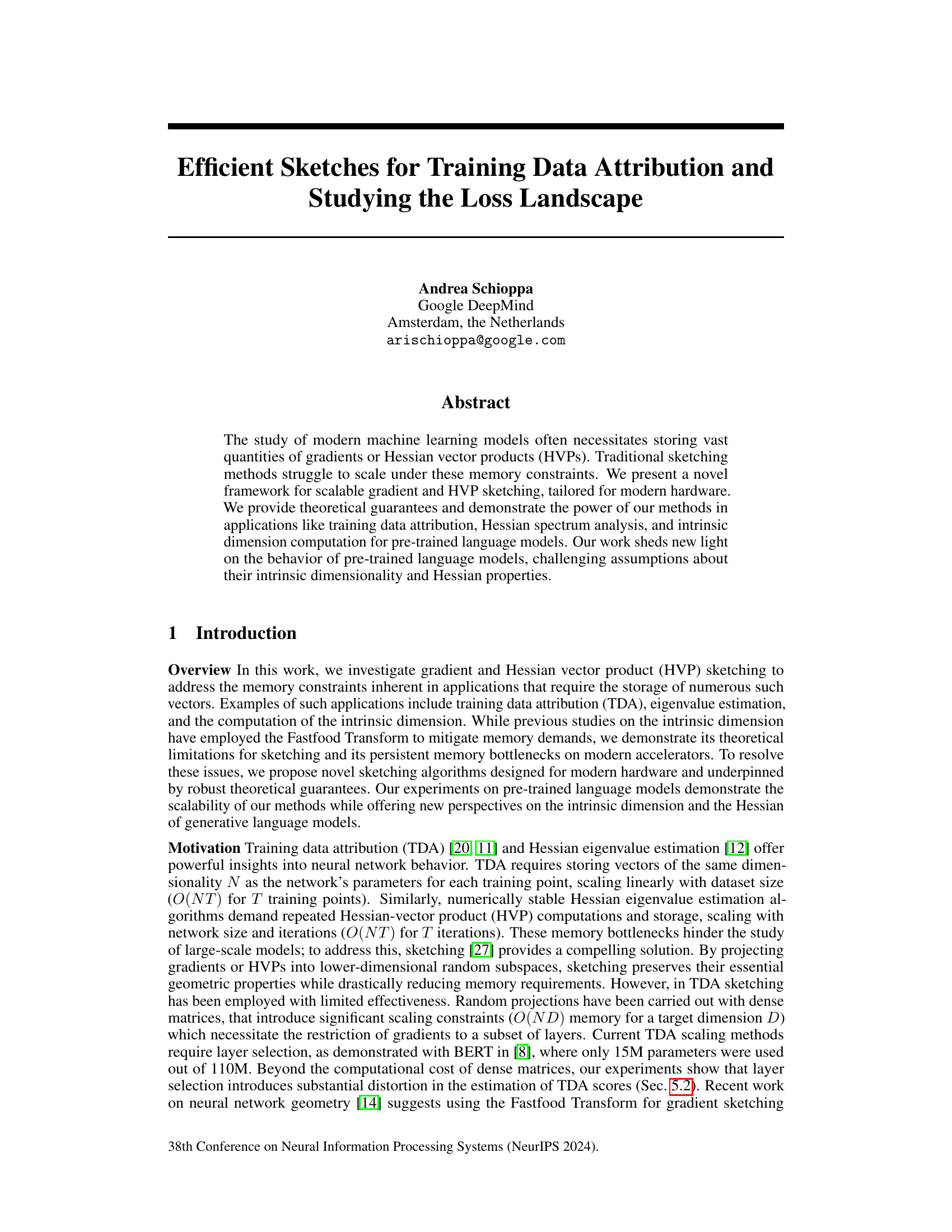
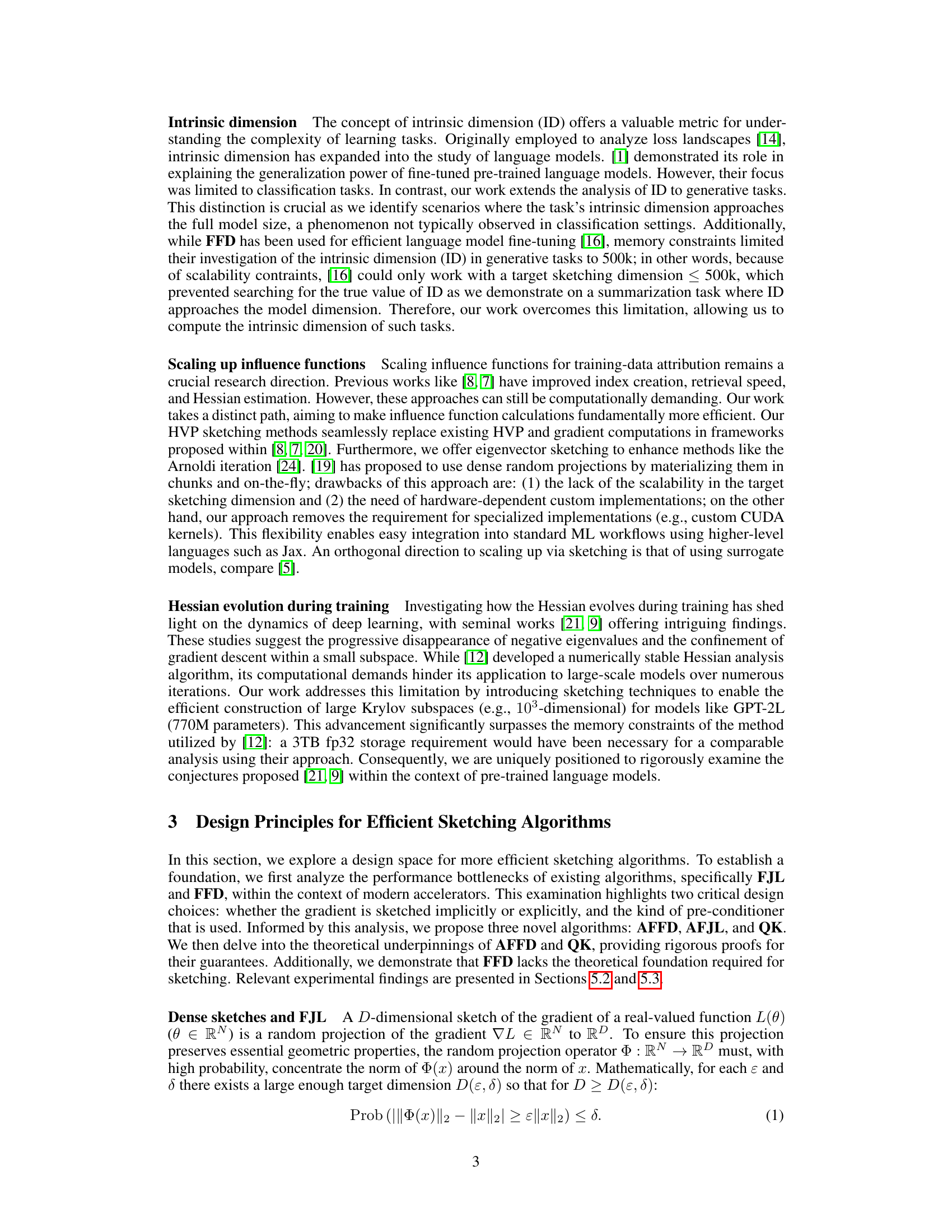
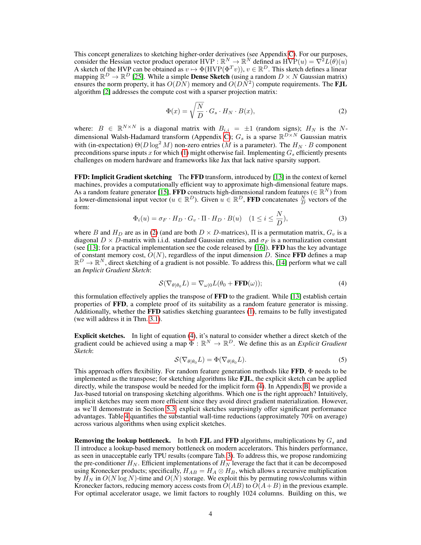
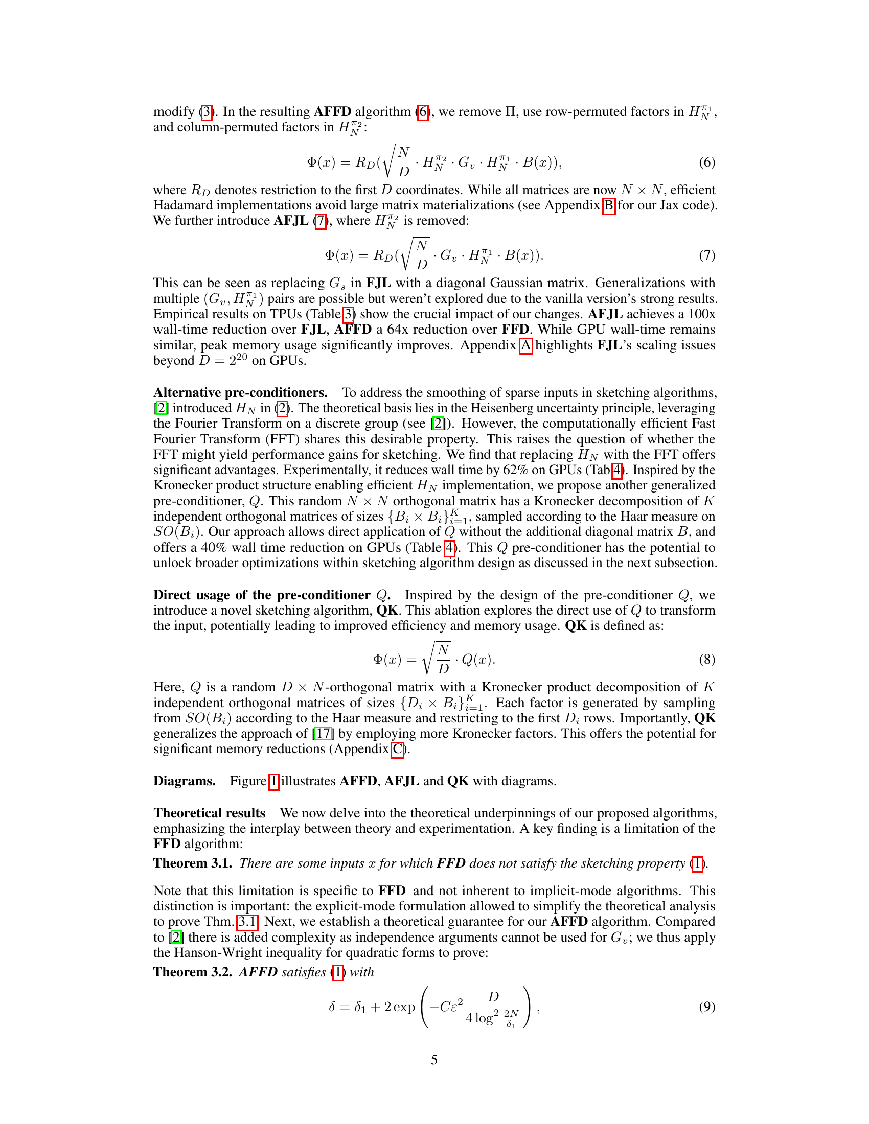
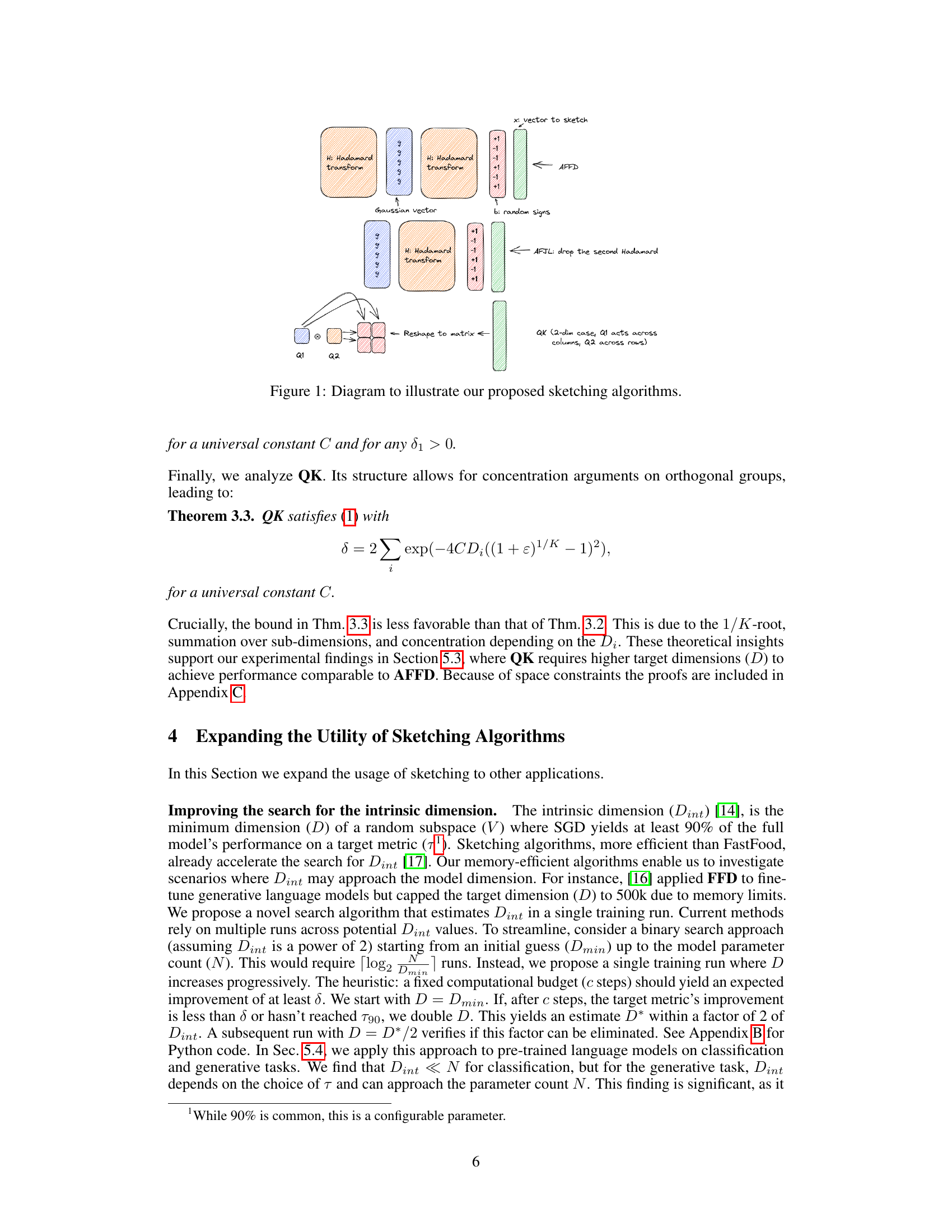
🔼 This figure illustrates the three novel sketching algorithms proposed in the paper: AFFD, AFJL, and QK. It shows the steps involved in each algorithm, highlighting the use of Hadamard transforms, Gaussian vectors, and Kronecker products. The diagram visually depicts the differences between the algorithms and how they achieve dimensionality reduction. AFFD uses two Hadamard transforms, AFJL uses one, and QK uses a Kronecker product decomposition of the input.
read the caption
Figure 1: Diagram to illustrate our proposed sketching algorithms.

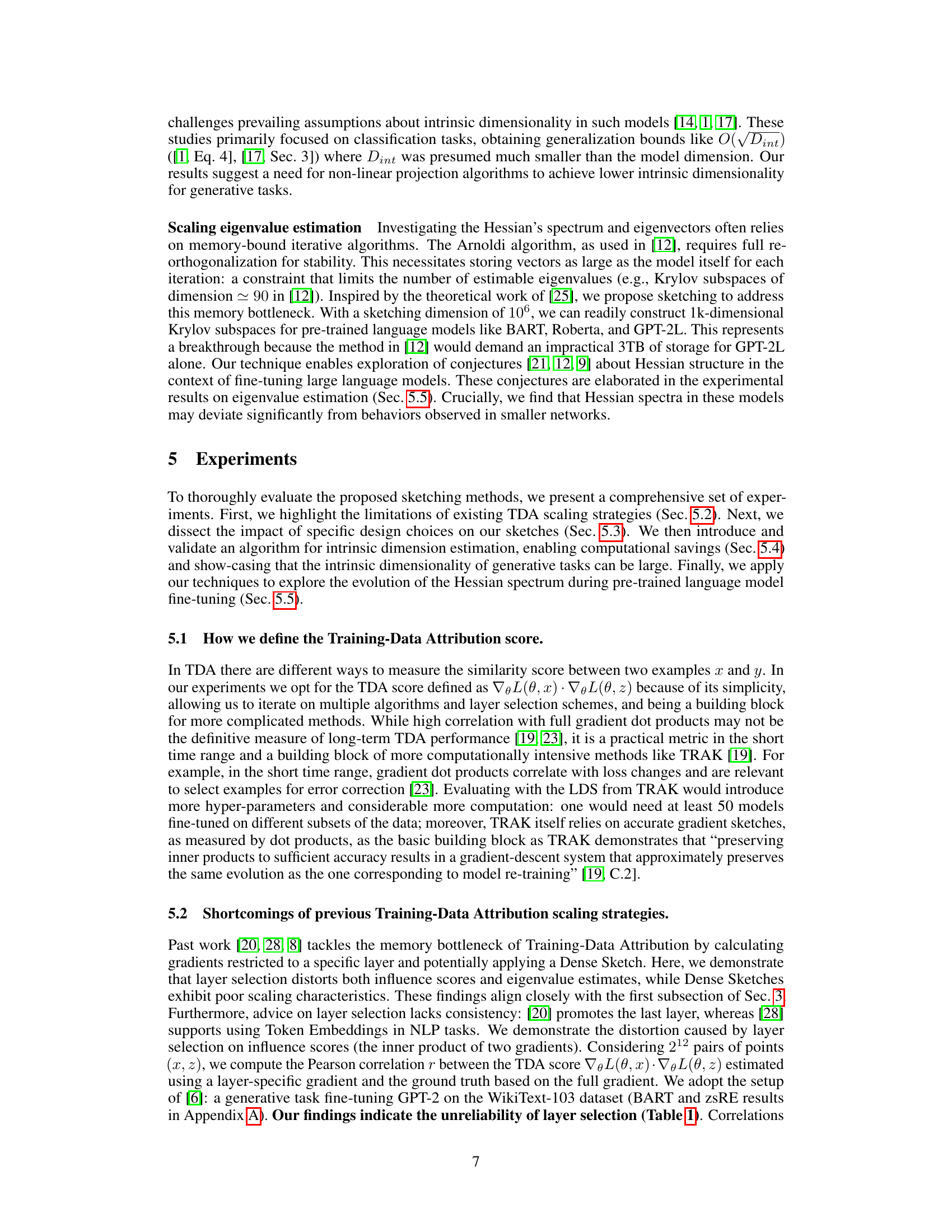
🔼 This table presents the results of an experiment evaluating the reliability of layer selection methods for training data attribution (TDA) and Hessian eigenvalue estimation. It shows that using only a subset of layers (instead of the entire model) produces significantly lower correlations with ground truth influence scores and higher errors in eigenvalue prediction, demonstrating the unreliability of layer-selection-based scaling strategies for these tasks.
read the caption
Table 1: Layer selection results in unreliable estimates for influence scores and eigenvalue estimation. The best correlation with ground truth influence scores does not exceed 90% and is quite low for most layers; the relative error in eigenvalue prediction is always at least 20%.
In-depth insights#
Gradient Sketching#
Gradient sketching is a crucial technique for scaling machine learning algorithms to massive datasets. It addresses the memory bottleneck inherent in storing and manipulating high-dimensional gradient vectors by projecting them into lower-dimensional spaces. This projection, while lossy, preserves essential geometric properties of the gradients, allowing for efficient computation of quantities like training data attribution and Hessian information. The key challenge lies in designing efficient sketching algorithms that balance dimensionality reduction with accuracy and computational speed. The paper explores this design space, highlighting the limitations of existing methods like the Fastfood Transform and proposing novel algorithms like AFFD and AFJL, which are optimized for modern hardware. These novel algorithms offer robust theoretical guarantees and demonstrate superior performance on GPUs and TPUs. They offer new possibilities for training data analysis, and enable the investigation of Hessian properties in large language models, leading to a deeper understanding of these complex systems. The findings challenge prevailing assumptions about intrinsic dimensionality and Hessian structure in LLMs, suggesting the need for new theoretical tools and algorithmic approaches.
TDA Scaling#
The paper delves into the challenges of scaling training data attribution (TDA) for large neural networks. Traditional TDA methods struggle with memory constraints, particularly when dealing with massive datasets and large model parameters. The authors highlight the limitations of existing methods, such as those relying on layer selection or dense random projections, which introduce significant distortion and scalability issues. The core problem is addressed by proposing novel sketching algorithms, providing a scalable solution. These algorithms leverage efficient pre-conditioning techniques and modern hardware acceleration, which are optimized to overcome performance bottlenecks. The theoretical guarantees for the effectiveness and efficiency of these algorithms are given. Empirical results demonstrate that the new approach significantly outperforms previous methods, allowing for the analysis of larger models and datasets, ultimately providing a more robust and scalable framework for understanding model behavior and training data influence.
Hessian Spectrum#
Analyzing the Hessian spectrum of large language models (LLMs) provides crucial insights into their training dynamics and generalization capabilities. Traditional methods struggle with the computational cost of Hessian computation for LLMs, necessitating the use of efficient sketching techniques. This allows for the estimation of the Hessian’s spectrum, revealing characteristics such as the distribution of eigenvalues, the presence of outliers, and the evolution of the spectrum during training. Studying the Hessian spectrum can reveal information about the intrinsic dimensionality of LLMs, challenging existing assumptions about the low dimensionality of the relevant parameter space. Furthermore, the presence and behavior of negative eigenvalues in the Hessian can provide insights into the optimization landscape and the effectiveness of training methods. The evolution of the Hessian spectrum during fine-tuning offers insights into how LLMs adapt to specific tasks, the emergence of dominant directions, and the relationship between Hessian structure and generalization performance. Overall, analyzing the Hessian spectrum is a powerful tool for gaining a deeper understanding of LLMs’ internal workings and their behavior during training and generalization.
LLM Geometry#
The term “LLM Geometry” evokes the study of the high-dimensional spaces within which large language models (LLMs) operate. Understanding this geometry is crucial for explaining LLMs’ behavior, such as their generalization ability, and for improving training and inference efficiency. Research in this area might explore the intrinsic dimensionality of the loss landscape, analyzing the distribution of gradients and Hessian matrices to uncover inherent structure. Key questions would involve identifying low-dimensional manifolds where most of the model’s learning dynamics occur, and whether this structure relates to the model’s performance on various tasks. Investigating the relationship between the geometry of the model’s parameter space and the semantic space it represents is another significant area. This might involve characterizing how similar sentences or concepts are represented by nearby points in parameter space, or how different tasks might occupy distinct regions of the space. Ultimately, a deep understanding of LLM Geometry will be essential for designing more efficient, robust, and interpretable LLMs.
Future Directions#
Future research could explore several promising avenues. Improving the theoretical understanding of sketching methods is crucial, particularly for handling non-i.i.d. data and complex model architectures. Developing more efficient algorithms for both gradient and Hessian sketching on diverse hardware platforms (including specialized accelerators) remains a key challenge. Extending the application of sketching techniques to other domains, such as reinforcement learning and causal inference, represents another significant opportunity. Finally, investigating the interplay between sketching and other model compression techniques (e.g., quantization, pruning) could lead to significant advances in model efficiency and scalability.
More visual insights#
More on figures

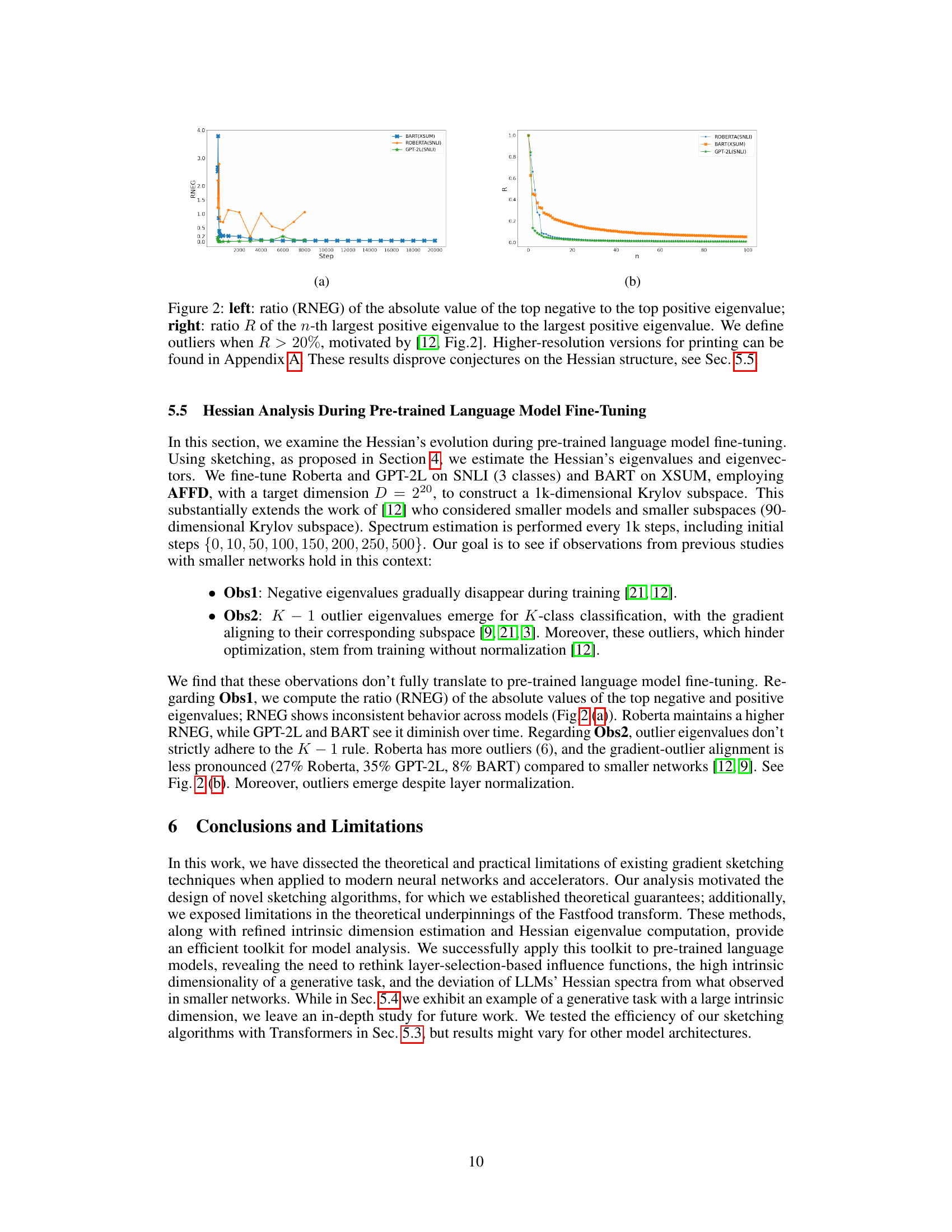
🔼 This figure shows two plots. The left plot displays the ratio of the absolute value of the top negative eigenvalue to the top positive eigenvalue (RNEG) over training steps. The right plot shows the ratio of the nth largest positive eigenvalue to the largest positive eigenvalue (R) against n (the rank). The plots illustrate that previously held assumptions about Hessian structure in smaller networks do not hold for large language models, specifically contradicting observations from prior research such as [12, Fig 2].
read the caption
Figure 2: left: ratio (RNEG) of the absolute value of the top negative to the top positive eigenvalue; right: ratio R of the n-th largest positive eigenvalue to the largest positive eigenvalue. We define outliers when R > 20%, motivated by [12, Fig.2]. Higher-resolution versions for printing can be found in Appendix A. These results disprove conjectures on the Hessian structure, see Sec. 5.5.
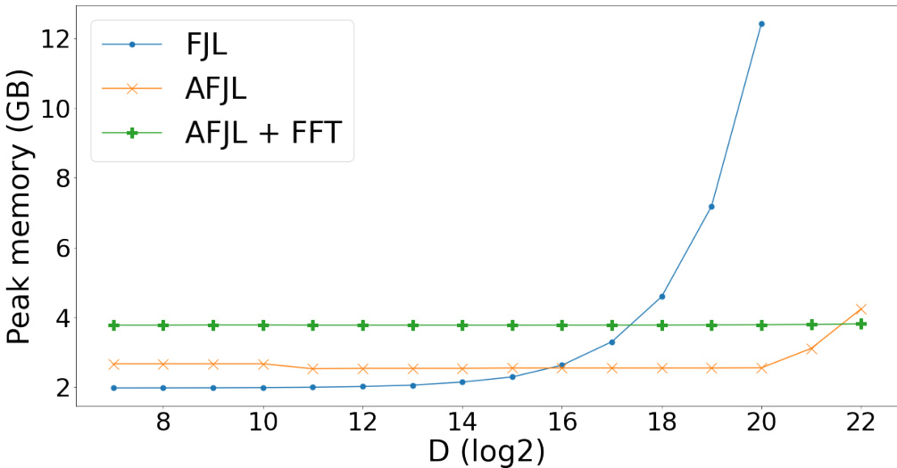
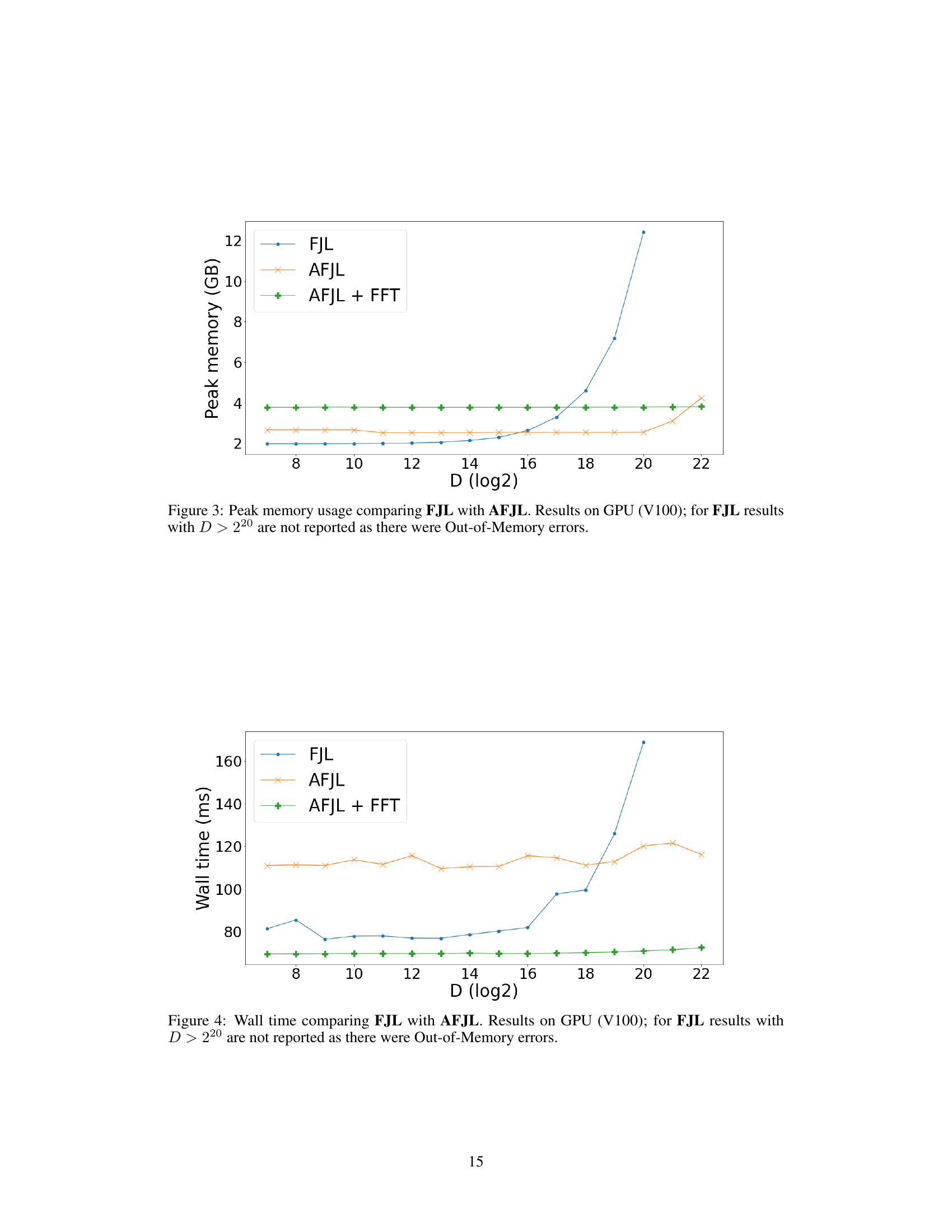
🔼 The figure shows a comparison of peak memory usage between FJL and AFJL algorithms on a GPU (V100) for different values of the target dimension D (log2 scale). It highlights the scalability issues with FJL, which experiences significant memory growth as D increases, resulting in out-of-memory errors beyond D=2^20. In contrast, AFJL demonstrates better scalability with relatively stable memory usage across the range of D values.
read the caption
Figure 3: Peak memory usage comparing FJL with AFJL. Results on GPU (V100); for FJL results with D > 220 are not reported as there were Out-of-Memory errors.
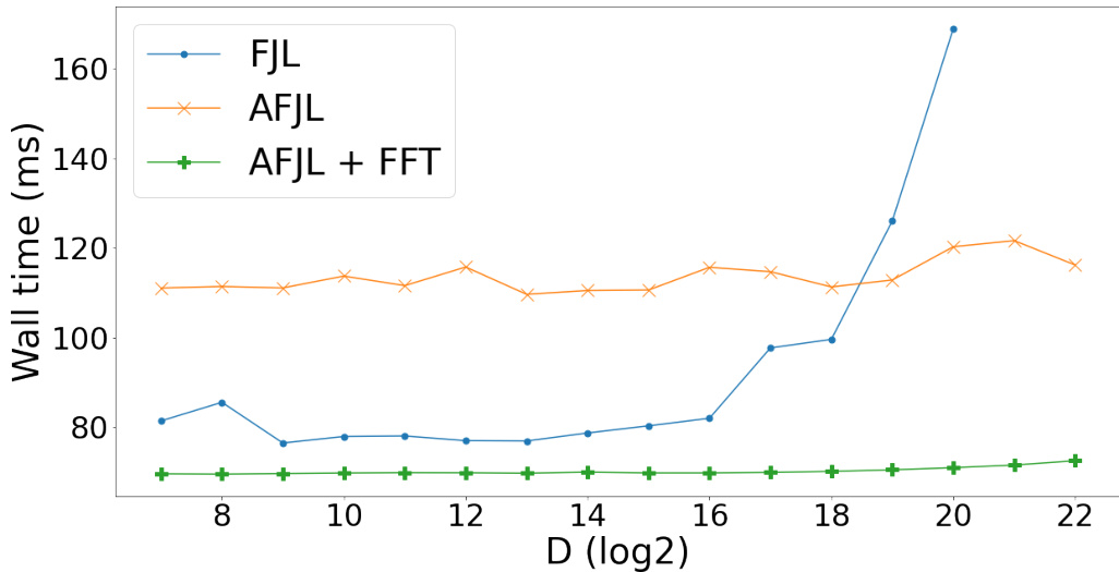
🔼 This figure compares the wall time of the FJL and AFJL algorithms for sketching gradients on a V100 GPU. The plot shows that AFJL is significantly faster than FJL, especially as the target dimension (D) increases. For larger values of D (above 220), FJL runs out of memory, highlighting the improved scalability of AFJL.
read the caption
Figure 4: Wall time comparing FJL with AFJL. Results on GPU (V100); for FJL results with D > 220 are not reported as there were Out-of-Memory errors.
🔼 This figure shows a comparison of three different sketching algorithms: AFFD, AFJL, and QK. It illustrates the steps involved in each algorithm, highlighting the use of Hadamard transforms, Gaussian matrices, and Kronecker products to efficiently sketch gradients. The figure also shows how the algorithms can be adapted for different types of sketches (explicit vs. implicit) and for different types of hardware (GPUs vs. TPUs).
read the caption
Figure 1: Diagram to illustrate our proposed sketching algorithms.
🔼 This figure provides a visual representation of the three novel sketching algorithms proposed in the paper: AFFD, AFJL, and QK. It shows how each algorithm processes the input gradient vector through a series of transformations involving Hadamard transforms and Gaussian matrices. The diagram highlights the key differences in the preconditioning steps and the explicit versus implicit sketching approaches, helping readers to better understand the algorithmic differences and their impact on efficiency.
read the caption
Figure 1: Diagram to illustrate our proposed sketching algorithms.

🔼 This figure shows two plots illustrating the Hessian’s evolution during pre-trained language model fine-tuning. The left plot displays the ratio of the absolute value of the top negative eigenvalue to the top positive eigenvalue (RNEG). The right plot shows the ratio of the nth largest positive eigenvalue to the largest positive eigenvalue (R). These ratios are calculated at various steps during the training process. An outlier is defined when the ratio R exceeds 20%. The figure provides insights into the Hessian structure, challenging earlier assumptions made in prior research.
read the caption
Figure 2: left: ratio (RNEG) of the absolute value of the top negative to the top positive eigenvalue; right: ratio R of the n-th largest positive eigenvalue to the largest positive eigenvalue. We define outliers when R > 20%, motivated by [12, Fig.2]. Higher-resolution versions for printing can be found in Appendix A. These results disprove conjectures on the Hessian structure, see Sec. 5.5.
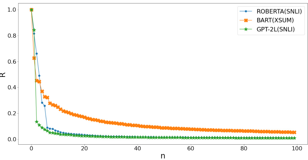
🔼 This figure displays two plots showing the ratio of eigenvalues of the Hessian matrix during the fine-tuning of pre-trained language models. The left plot shows the ratio of the absolute value of the top negative eigenvalue to the top positive eigenvalue (RNEG), while the right plot shows the ratio of the nth largest positive eigenvalue to the largest positive eigenvalue (R). The plots illustrate that previous conjectures regarding Hessian structure in smaller networks do not hold true for large language models.
read the caption
Figure 2: left: ratio (RNEG) of the absolute value of the top negative to the top positive eigenvalue; right: ratio R of the n-th largest positive eigenvalue to the largest positive eigenvalue. We define outliers when R > 20%, motivated by [12, Fig.2]. Higher-resolution versions for printing can be found in Appendix A. These results disprove conjectures on the Hessian structure, see Sec. 5.5.
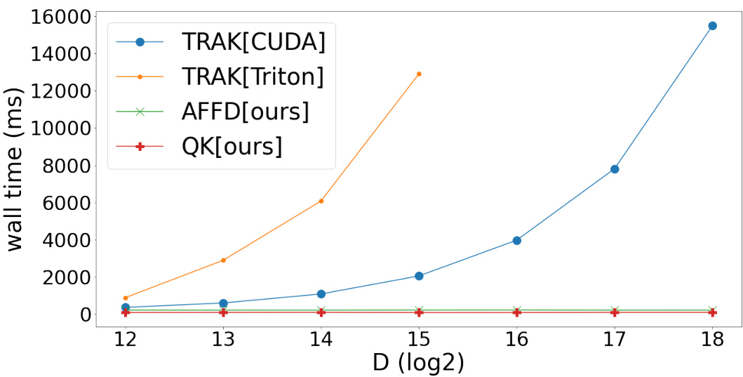
🔼 This figure compares the wall time performance of different gradient sketching algorithms. It shows that the proposed methods (AFFD and QK) exhibit constant wall time regardless of the target dimension (D), while the competing method (TRAK) shows a significant increase in runtime as D increases. The performance difference between two different implementations of the TRAK algorithm (CUDA and Triton) highlights the difficulty in efficiently implementing dense random projections.
read the caption
Figure 7: Our methods exhibit constant wall time with respect to the target dimension D. In contrast, TRAK's runtime increases with the target dimension. Efficient implementation of dense random projections with recomputed projectors is non-trivial; compare the performance difference between TRAK[CUDA] and TRAK[Triton]. TRAK[CUDA] utilizes the CUDA kernel provided by the original TRAK authors [19].

🔼 This figure shows a comparison of three different sketching algorithms: AFFD, AFJL, and QK. It illustrates the steps involved in each algorithm, highlighting the differences in their approaches to sketching gradients or Hessian vector products. The diagram details how each algorithm uses Hadamard transforms, Gaussian matrices, and Kronecker products to perform the sketching operation. The visualization helps readers understand the computational cost and memory requirements of each method, emphasizing their unique design choices and their relative efficiency.
read the caption
Figure 1: Diagram to illustrate our proposed sketching algorithms.
More on tables

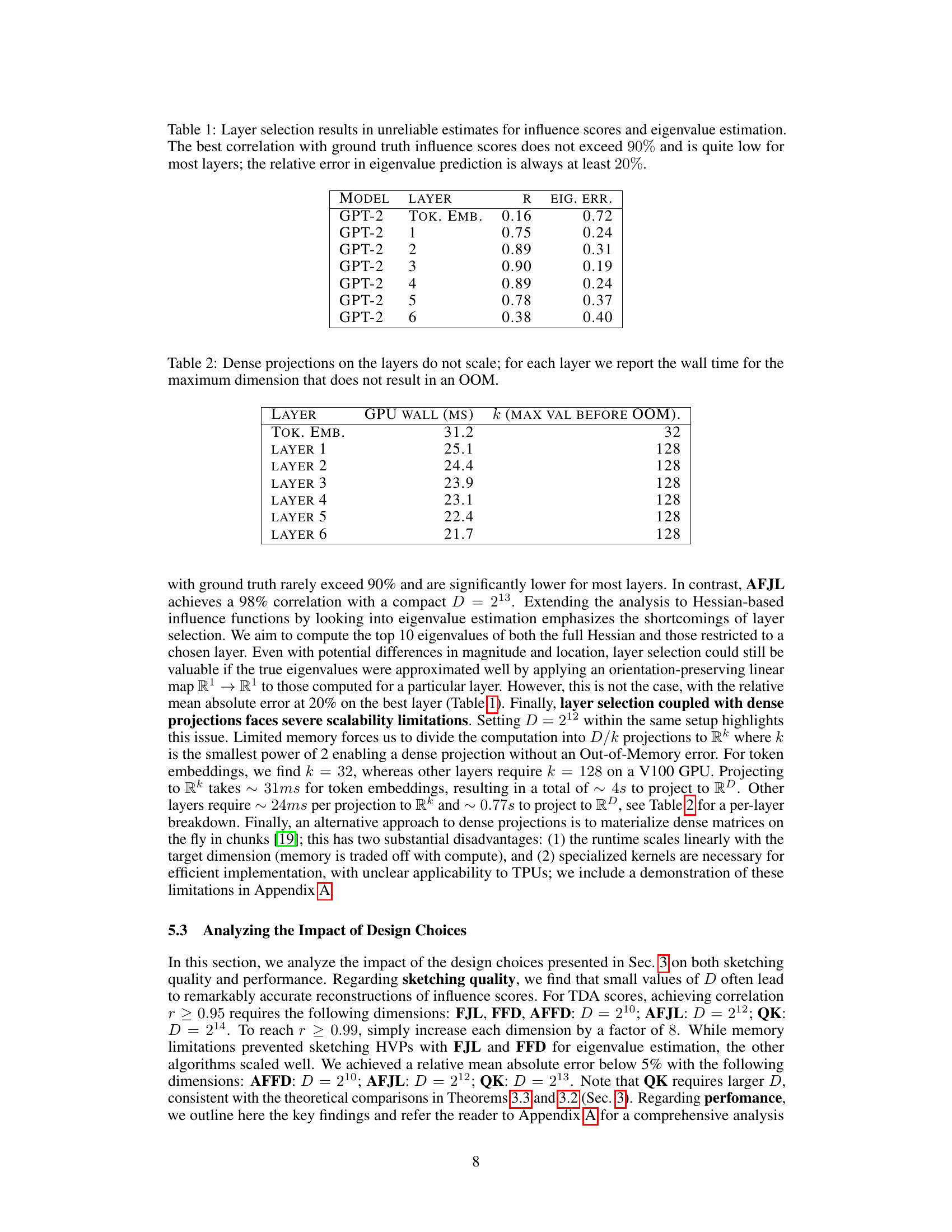
🔼 This table presents the results of an experiment evaluating the scalability of dense projections on different layers of a neural network. For each layer, it shows the wall time (in milliseconds) taken for computation with the maximum dimension that did not lead to an out-of-memory (OOM) error. The results demonstrate that dense projections are not scalable as the maximum dimension that fits in memory decreases with each subsequent layer.
read the caption
Table 2: Dense projections on the layers do not scale; for each layer we report the wall time for the maximum dimension that does not result in an OOM.

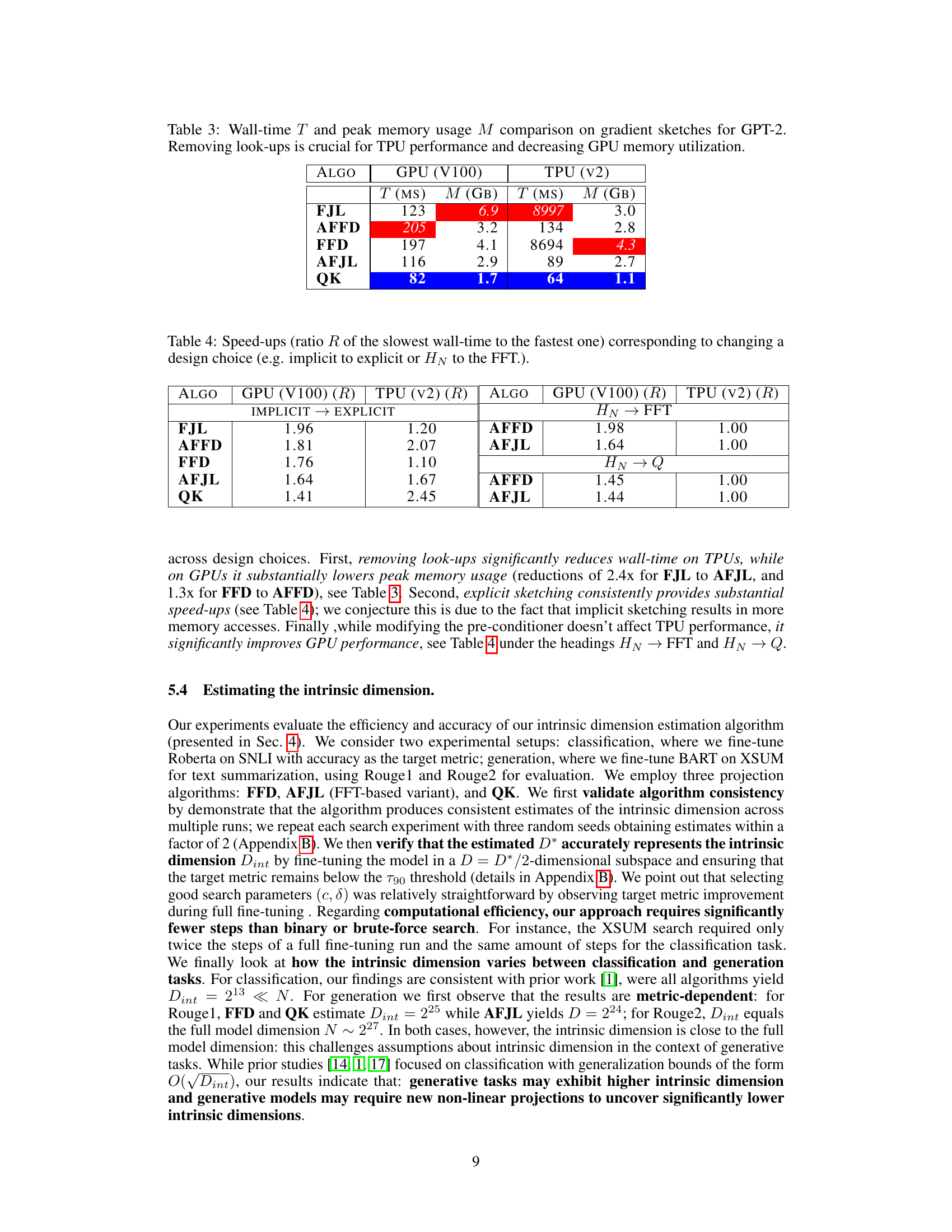
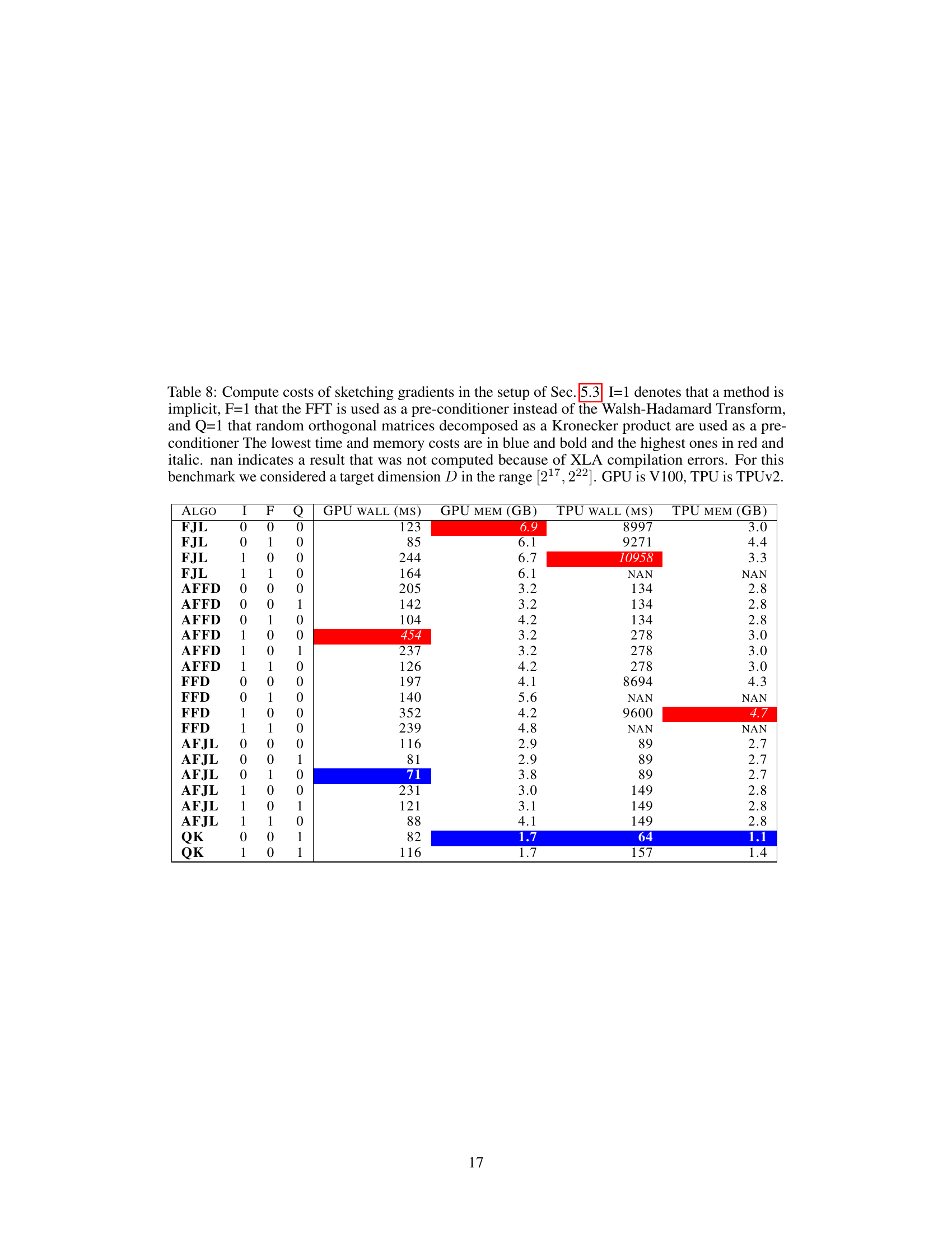
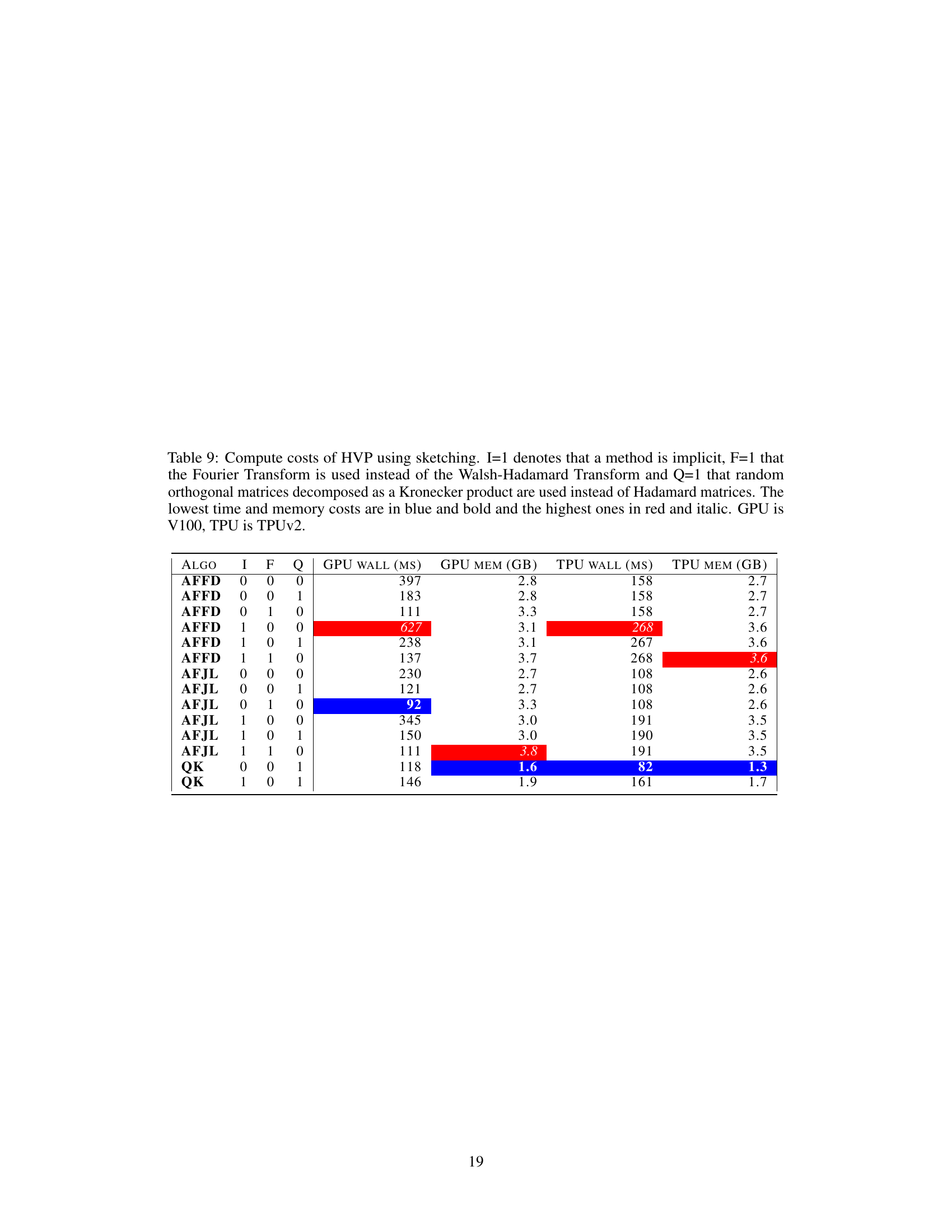
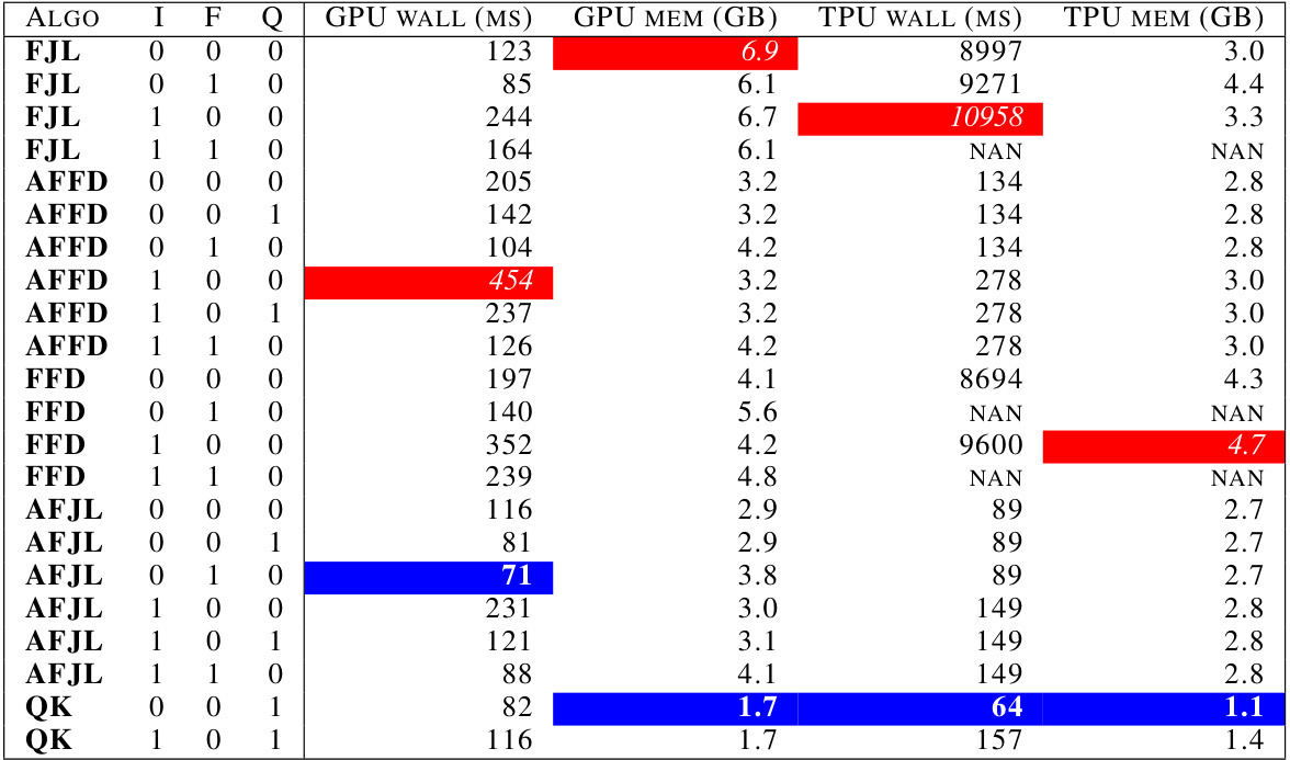
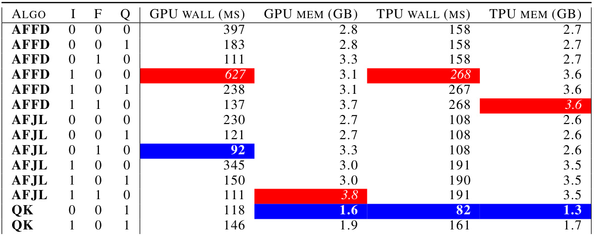
🔼 This table compares the wall-time and peak memory usage of different gradient sketching algorithms (FJL, AFFD, FFD, AFJL, QK) for GPT-2 on both GPU (V100) and TPU (v2) hardware. The results show the impact of removing lookups, a key optimization in the proposed algorithms, on both performance metrics. Lower values of T (wall-time in milliseconds) and M (memory in gigabytes) are better, indicating faster and more memory-efficient algorithms.
read the caption
Table 3: Wall-time T and peak memory usage M comparison on gradient sketches for GPT-2. Removing look-ups is crucial for TPU performance and decreasing GPU memory utilization.

🔼 This table shows the speedup achieved by changing specific design choices in the sketching algorithms. The speedup is calculated as the ratio of the slowest wall time to the fastest wall time for each algorithm and hardware (GPU or TPU). The design choices evaluated include switching from implicit to explicit sketching, and replacing the Walsh-Hadamard transform (HN) with either the Fast Fourier Transform (FFT) or a Kronecker-product-based orthogonal matrix (Q).
read the caption
Table 4: Speed-ups (ratio R of the slowest wall-time to the fastest one) corresponding to changing a design choice (e.g. implicit to explicit or HN to the FFT.).
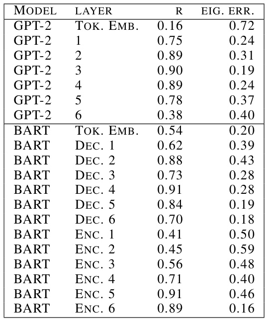
🔼 This table presents the Pearson correlation (R) between influence scores obtained using layer-specific gradients and the ground truth (full gradient) for various layers in GPT-2 and BART models, along with the relative error in eigenvalue estimation for each layer. The results show that layer selection leads to unreliable estimates for both influence scores and eigenvalues. Correlations with the ground truth are generally below 90%, and the relative error in eigenvalue prediction is always at least 20%. This highlights the unreliability of layer selection as a scaling strategy for training data attribution.
read the caption
Table 1: Layer selection results in unreliable estimates for influence scores and eigenvalue estimation. The best correlation with ground truth influence scores does not exceed ~90% and is quite low for most layers; the relative error in eigenvalue prediction is always at least ~20%.
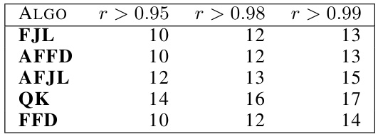
🔼 This table presents the minimum log2(D) values required for different sketching algorithms (FJL, AFFD, AFJL, QK, FFD) to achieve Pearson correlation (r) values exceeding 0.95, 0.98, and 0.99 when estimating inner products of gradients. It shows the relationship between the target dimension D and the accuracy of the gradient sketching methods in approximating inner products.
read the caption
Table 6: For each algorithm the minimal value of log2 D necessary to reach a Pearson r > x where x = 0.9{5,8,9} for estimating inner products of gradients.

🔼 This table shows the minimum log2(D) values required for AFFD, AFJL, and QK algorithms to achieve relative errors of less than 0.2, 0.1, and 0.05 when reconstructing the top 10 Hessian eigenvalues. It demonstrates the different memory requirements for achieving similar accuracy with different sketching algorithms.
read the caption
Table 7: For each algorithm the minimal value of log2 D necessary to reach a relative error err < x where x = 0.2, 0.1, 0.05 in reconstructing the top 10 eigenvalues.

🔼 This table shows the stability of the algorithm used to search for the intrinsic dimension (D*). For each task (SNLI, XSUM) and metric (accuracy, ROUGE1), the algorithm ran three times with different random seeds. The table displays the resulting D* values for each run. The results show that the D* values are consistent within a factor of 2 across different seeds, demonstrating the algorithm’s stability.
read the caption
Table 10: Values of D* returned by the search the intrinsic dimension Dint using 3 different seeds. This shows the stability of our algorithm which doubles the dimension of the fine-tuning subspace after some compute budget if the target metric has not improved enough.

🔼 This table compares the wall-time performance of three different sketching algorithms (AFFD, QK, and TRAK) on a V100 GPU for various target dimensions. TRAK, which uses on-the-fly dense random projections, shows a significant increase in wall-time as the target dimension increases, while AFFD and QK maintain relatively constant runtimes.
read the caption
Table 11: Wall-time T (ms) Comparison: Our Methods vs. On-the-fly Dense Projections (TRAK) using a V100 GPU. TRAK requires custom kernels and is thus restricted to GPU computation. Our methods exhibit constant runtime with respect to the target dimension, whereas TRAK's runtime increases substantially as the target dimension grows.
Full paper#
