TL;DR#
A computational challenge in reward-based learning is how the brain coordinates learning using distributed error signals, unlike the sequential backpropagation method used in artificial neural networks. The paper addresses this by proposing that distributed, per-layer TD errors can suffice, challenging the prevailing notion that sequential error signaling is necessary.
The proposed solution, called Artificial Dopamine (AD), is a deep Q-learning algorithm that leverages per-layer predictions and locally homogenous errors mimicking the biological dopamine distribution. Forward connections between layers also enable information exchange without error backpropagation. Experiments on various RL tasks show AD’s performance is comparable to algorithms using backpropagation, highlighting the potential of distributed error signals for effective learning. This challenges existing deep RL paradigms and offers a more biologically plausible approach.
Key Takeaways#
Why does it matter?#
This paper is crucial because it challenges the conventional wisdom in deep reinforcement learning by demonstrating that complex tasks can be solved using only locally distributed error signals, mirroring biological systems. This opens new avenues for developing more biologically plausible and efficient algorithms, potentially leading to significant energy savings and improved performance.
Visual Insights#

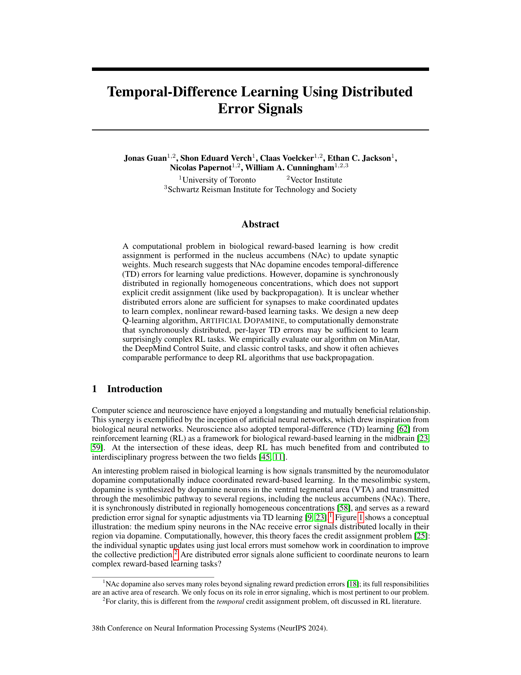
🔼 This figure illustrates the pathway of dopamine from the ventral tegmental area (VTA) to the nucleus accumbens (NAc). Dopamine neurons in the VTA synthesize dopamine and transport it along their axons to the NAc. In the NAc, dopamine is released and picked up by receptors on medium spiny neurons. The concentration of dopamine is relatively homogeneous within local regions of the NAc, but can vary across different regions. The figure simplifies the complex neural connections in the NAc for clarity.
read the caption
Figure 1: Simplified illustration of dopamine distribution in the NAc. Dopamine is synthesized in the VTA and transported along axons to the NAc, where it is picked up by receptors in medium spiny neurons. Dopamine concentrations (error signals) are locally homogenous, but can vary across regions. Connections between NAc neurons not shown.

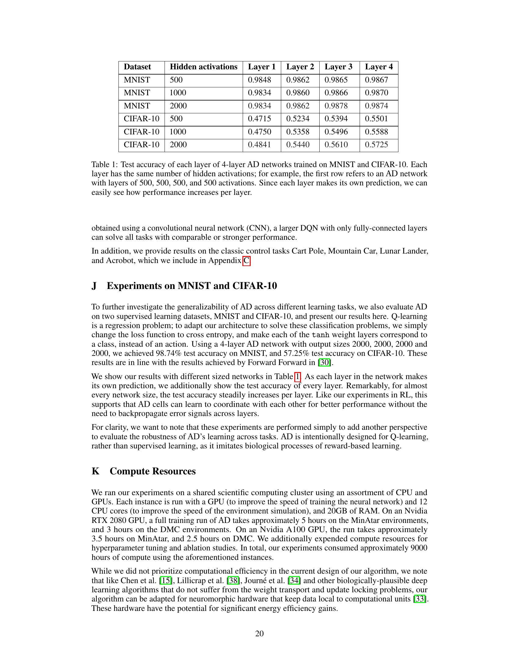
🔼 This table presents the test accuracy achieved by each layer in a 4-layer Artificial Dopamine (AD) network trained on the MNIST and CIFAR-10 datasets. Each layer of the network has an identical number of hidden activations. The table demonstrates how the model’s performance improves layer by layer, as each layer produces its own prediction.
read the caption
Table 1: Test accuracy of each layer of 4-layer AD networks trained on MNIST and CIFAR-10. Each layer has the same number of hidden activations; for example, the first row refers to an AD network with layers of 500, 500, 500, and 500 activations. Since each layer makes its own prediction, we can easily see how performance increases per layer.
In-depth insights#
Dopamine’s Role#
The paper explores dopamine’s crucial role in biological reward-based learning, focusing on its function in the nucleus accumbens (NAc). Research suggests dopamine signals temporal-difference (TD) errors, crucial for updating synaptic weights, thus enabling learning of value predictions. However, dopamine’s synchronous distribution challenges the traditional view of explicit credit assignment, as seen in backpropagation. The authors investigate if this distributed error signal is sufficient for coordinated synaptic updates in complex learning tasks. This is a key question addressed by their novel deep Q-learning algorithm, which uses distributed per-layer TD errors. The study’s findings suggest that synchronously distributed errors alone might be sufficient for effective learning, even in complex scenarios, thereby offering a computationally plausible model for how dopamine facilitates learning in the brain. This challenges the assumption that sequential error propagation, like in backpropagation, is necessary for credit assignment. The research provides compelling evidence that biological learning mechanisms might be more efficient and parallel than current artificial deep learning methods.
AD Algorithm#
The core of this research paper revolves around the Artificial Dopamine (AD) algorithm, a novel deep Q-learning method designed to mimic the distributed nature of dopamine in the brain’s reward system. Unlike traditional deep RL algorithms that rely on backpropagation, AD uses only synchronously distributed, per-layer temporal-difference (TD) errors. This approach tackles the credit assignment problem inherent in biological reward learning by avoiding the biologically implausible sequential error propagation found in backpropagation. The algorithm’s architecture, comprised of AD cells, is inspired by the Forward-Forward algorithm but adapted for value prediction in a Q-learning setting. The AD cell utilizes an attention mechanism, allowing for nonlinearity in value estimation without relying on error propagation between layers. Empirical results on various tasks demonstrate that AD often achieves comparable performance to deep RL algorithms that use backpropagation, suggesting that distributed errors alone may be sufficient for coordinated learning in complex tasks. This innovative approach opens exciting avenues for research at the intersection of neuroscience and artificial intelligence, offering a potentially more biologically plausible alternative to traditional deep reinforcement learning.
Benchmark Results#
A dedicated ‘Benchmark Results’ section would ideally present a thorough comparison of the novel algorithm’s performance against established baselines across various tasks. Key aspects to cover would include quantitative metrics (e.g., average reward, success rate, learning speed), statistical significance testing to validate performance differences, and a detailed analysis of results across different task types and complexities. Visualizations such as graphs and tables are essential for clear presentation of the data. A compelling analysis should not merely state the results but also interpret their implications. For instance, is the new algorithm consistently better or are improvements task-specific? Do the results support the authors’ hypotheses and contribute to the broader understanding of the problem? Are there any unexpected findings? A robust analysis would address these questions, leading to a deeper understanding of the algorithm’s strengths and weaknesses.
Forward Connections#
The concept of ‘forward connections’ in the context of Artificial Dopamine (AD) is crucial for enabling efficient learning with only distributed, per-layer temporal difference (TD) errors. Unlike backpropagation, which relies on backward error signals, AD utilizes forward connections to transmit information from upper layers to lower layers via activations rather than error signals. This design choice, inspired by the brain’s information processing, avoids the dependency and sequential processing inherent in backpropagation. The forward connections provide a pathway for upper layers to communicate useful representations to lower layers, promoting coordination and improving overall performance. This is particularly important for complex tasks where independently trained layers may not be sufficient for efficient learning. Empirical results demonstrate the significant improvement brought by forward connections, suggesting that such mechanisms might be part of the biological credit assignment process. The biological plausibility of this approach suggests that forward connections might be a key element of the brain’s reward-based learning system, and this feature of AD might offer avenues to explore new AI architectures inspired by neuroscience.
Study Limitations#
A thoughtful analysis of a research paper’s limitations section requires a nuanced approach. It’s crucial to consider what aspects the study doesn’t address, methodological shortcomings, and how these affect the conclusions. For example, were there sample size limitations or potential biases in data collection? Were certain variables controlled for or were there confounding factors? A good limitations section acknowledges such issues transparently, explaining the implications for the study’s generalizability and external validity. Furthermore, future research directions should be suggested, based on the identified limitations. This shows the researchers’ critical self-reflection and commitment to advancing the field. A strong limitations section doesn’t merely list weaknesses; it analyzes their potential impact on the results, promoting responsible interpretation and setting the stage for more robust future investigations. It demonstrates academic integrity and intellectual honesty.
More visual insights#
More on figures

🔼 This figure illustrates the architecture of a three-layer Artificial Dopamine (AD) network. Each layer contains an AD cell which computes its own local temporal difference (TD) error and updates its weights independently of other layers. There’s no backpropagation of error signals between layers. Information is passed forward in time from upper layers to lower layers using activations, not errors. The diagram shows how the activations (ht) are passed to AD cells across timesteps (t).
read the caption
Figure 2: Network architecture of a 3-layer AD network. ht represents the activations of layer l at time t, and st the input state. The blocks are AD cells, as shown in Figure 3. Similar to how dopamine neurons compute and distribute error used by a local region, each cell computes its own local TD error used by its updates; errors do not propagate across layers. To relay information, upper layers send activations to lower layers in the next timestep. For example, red shows all active connections at t = 1.

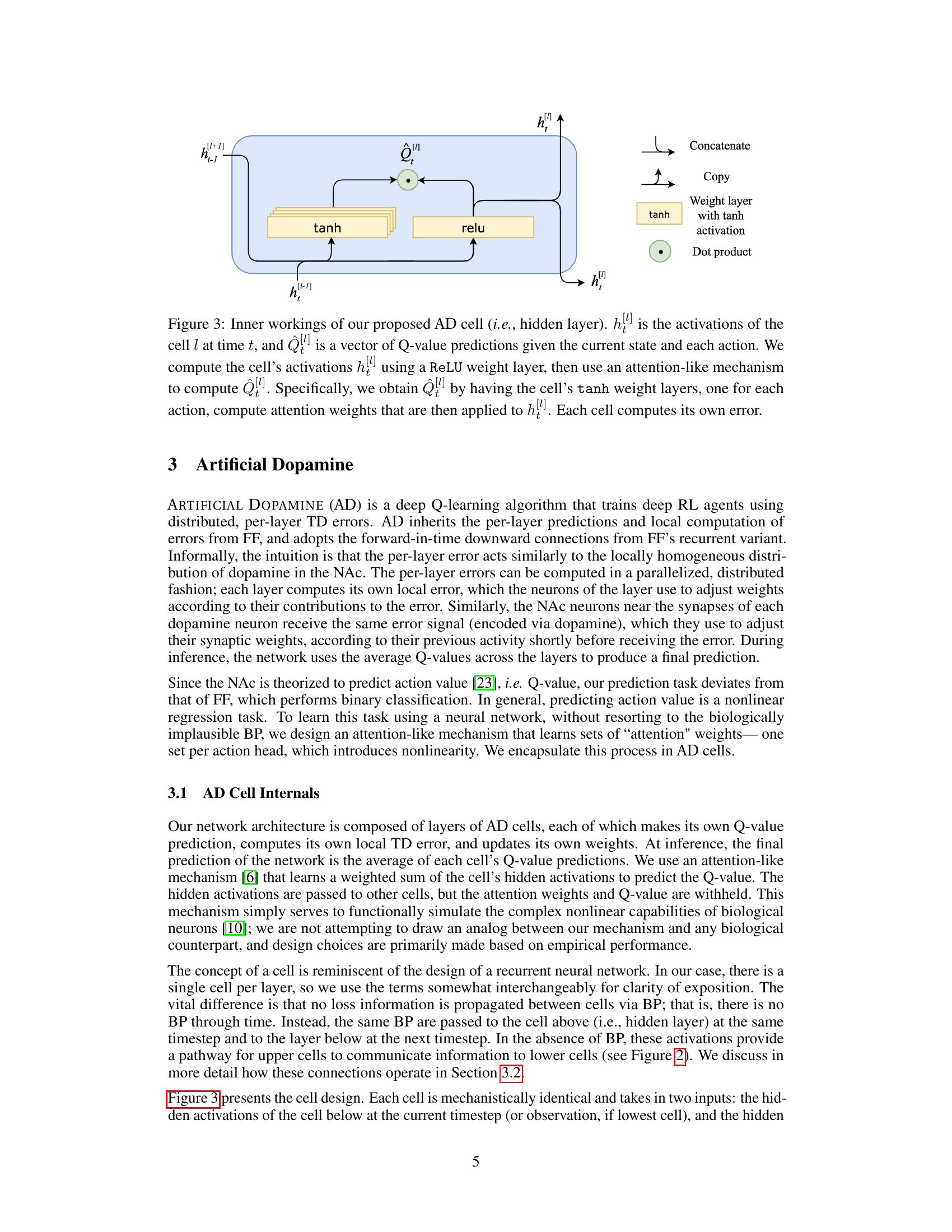
🔼 This figure details the internal structure and computations of a single Artificial Dopamine (AD) cell, a core component of the proposed deep Q-learning algorithm. The AD cell takes as input the hidden layer activations from the previous timestep from the layer above (h[l+1]t-1) and the current timestep from the layer below (h[l-1]t). It uses these inputs with multiple tanh and ReLU layers, and an attention mechanism to compute its Q-value predictions (Q[l]t) for each action. Importantly, each cell independently computes its own error, mirroring the local nature of dopamine signals in the brain’s reward system.
read the caption
Figure 3: Inner workings of our proposed AD cell (i.e., hidden layer). ht is the activations of the cell l at time t, and Q is a vector of Q-value predictions given the current state and each action. We compute the cell's activations h using a ReLU weight layer, then use an attention-like mechanism to compute Q. Specifically, we obtain Q by having the cell's tanh weight layers, one for each action, compute attention weights that are then applied to h. Each cell computes its own error.

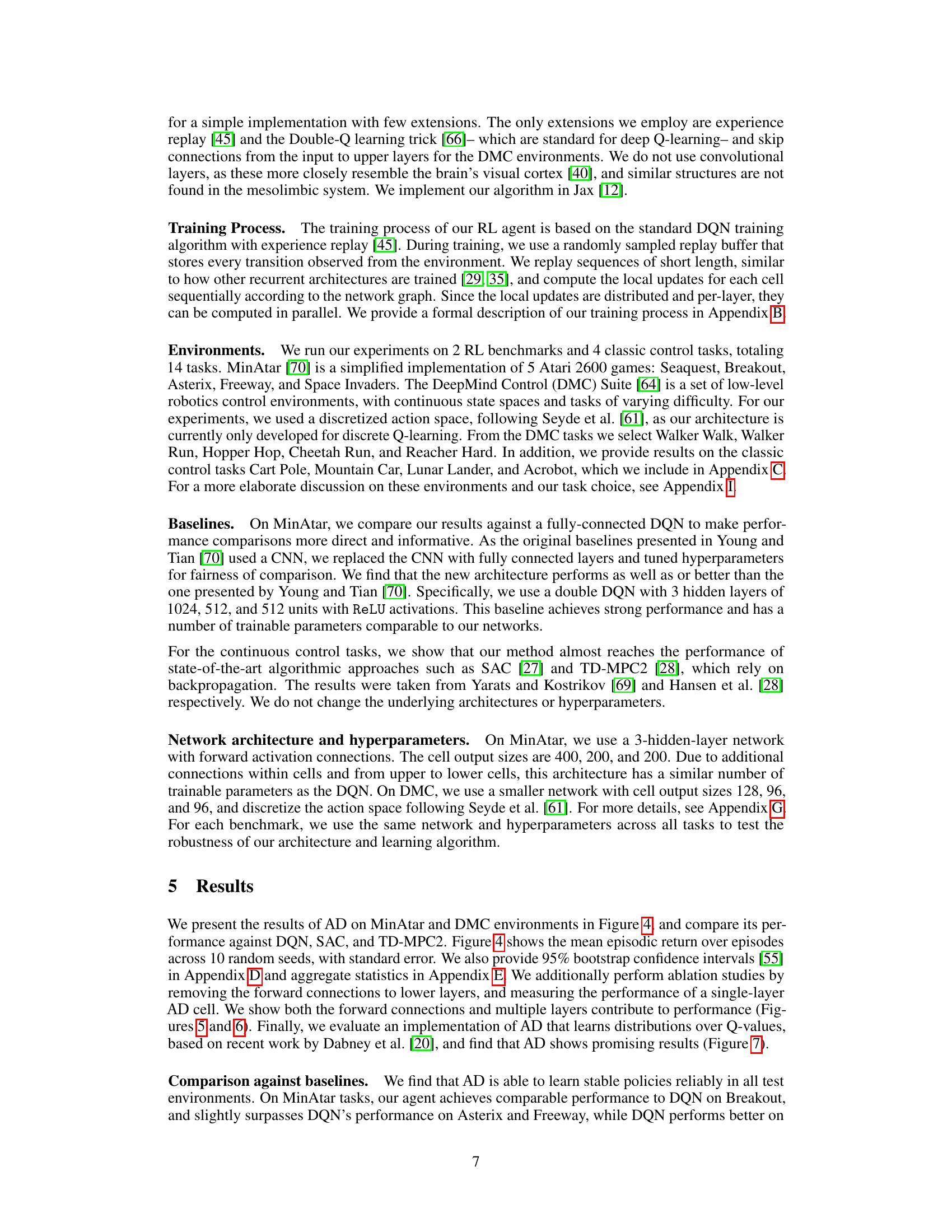
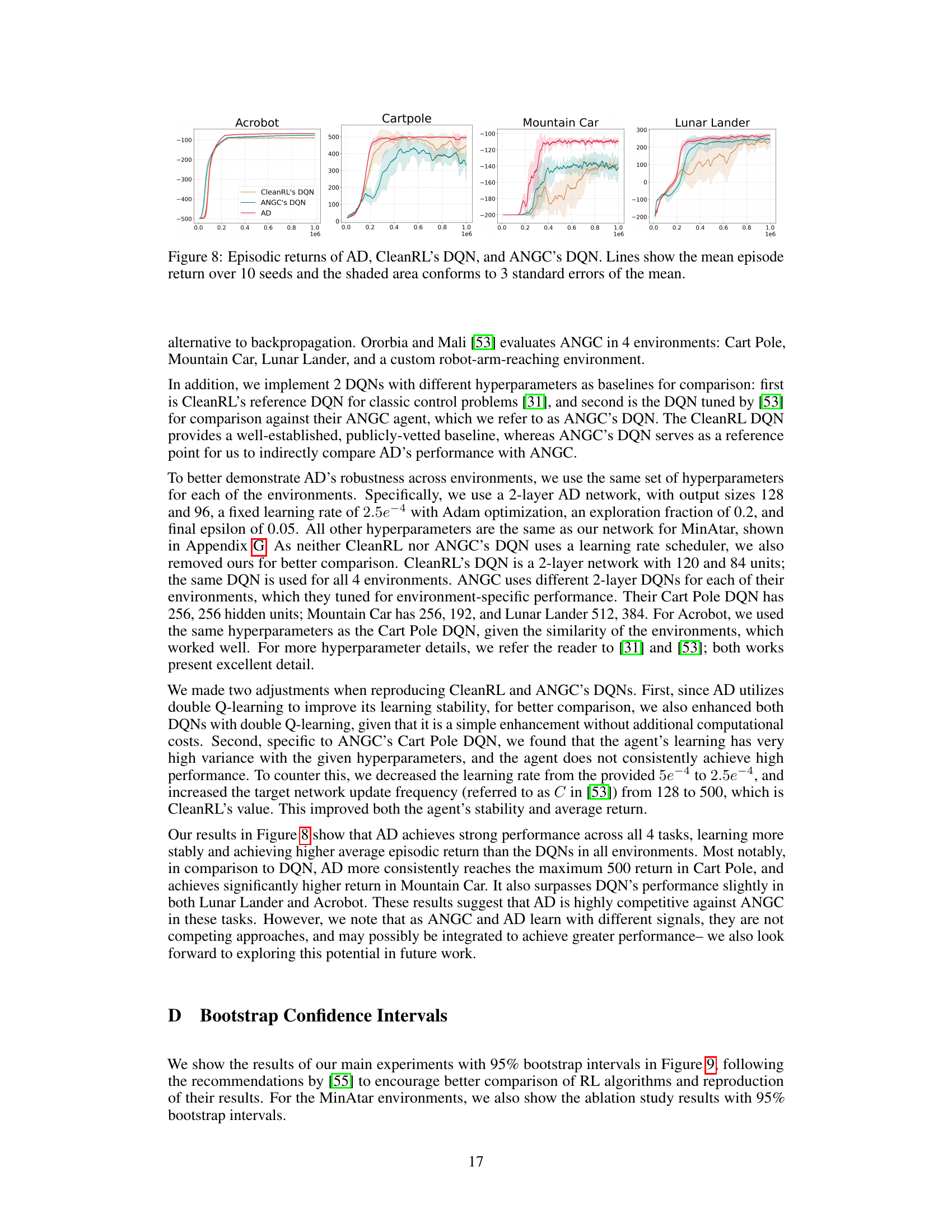
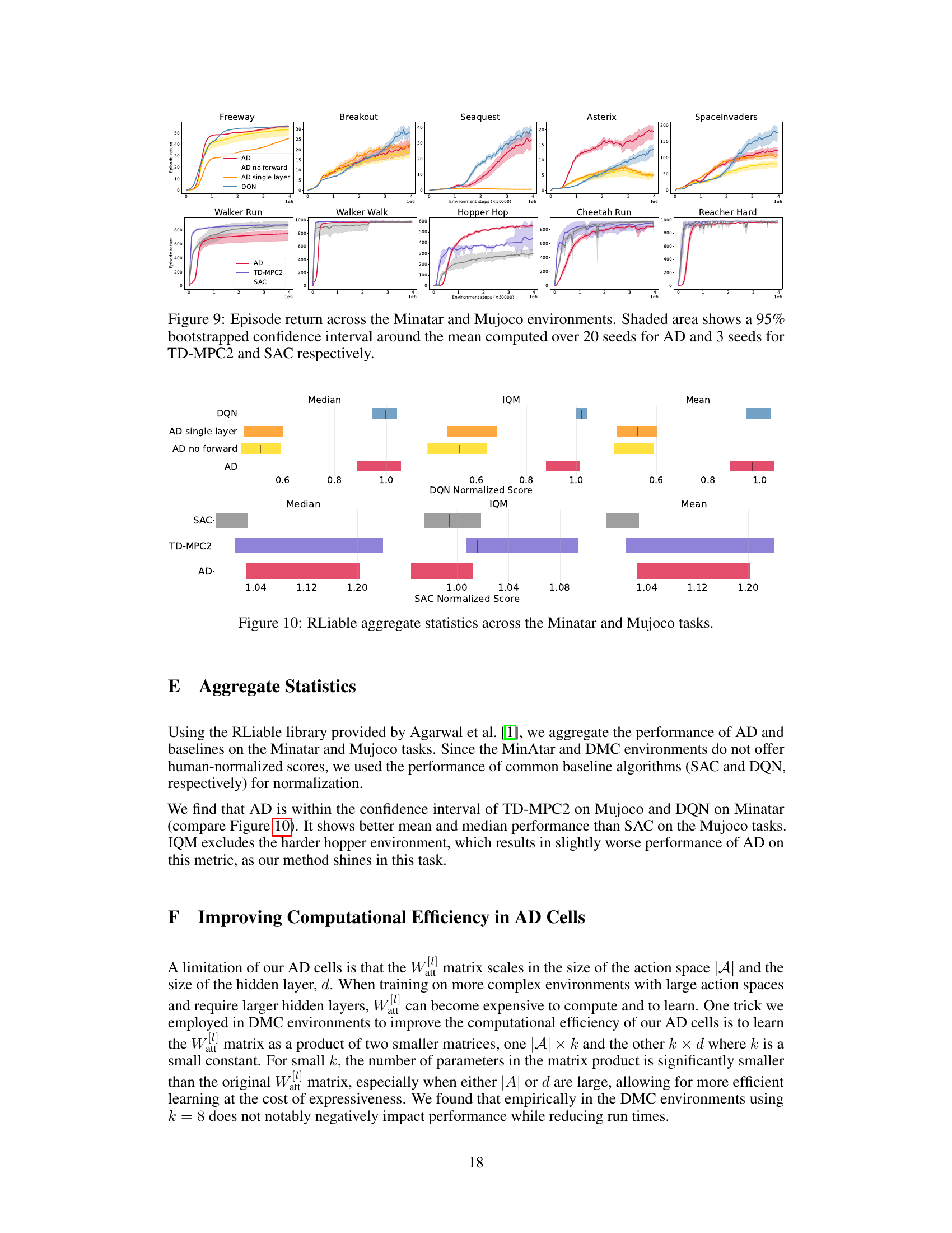
🔼 This figure presents the results of the Artificial Dopamine (AD) algorithm on a range of reinforcement learning tasks, comparing its performance to existing state-of-the-art algorithms. The tasks come from the MinAtar (discrete) and DeepMind Control (DMC) suites (continuous). For each task, the average episodic return is plotted over the course of training for AD, DQN (Deep Q-Network), TD-MPC2 (Temporal Difference Model Predictive Control), and SAC (Soft Actor-Critic). Error bars representing three standard errors are included to show the variability in performance across multiple runs.
read the caption
Figure 4: Episodic returns of AD in MinAtar and DMC environments, compared to DQN, TD-MPC2 and SAC. Lines show the mean return over 10 seeds and the shaded area conforms to 3 standard errors. The axes are return and environmental steps.

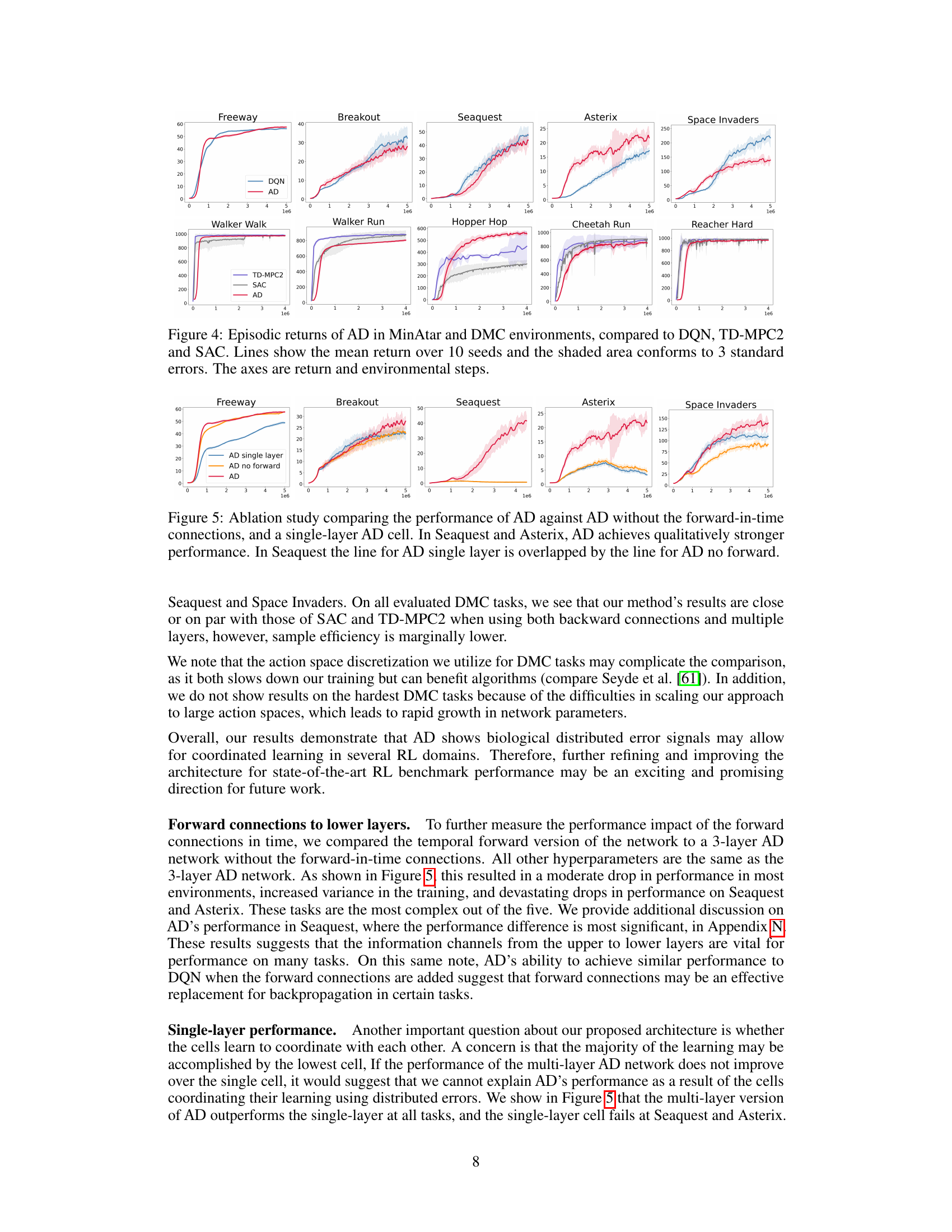
🔼 This figure presents an ablation study to evaluate the impact of the forward-in-time connections and multiple layers in the AD architecture. It compares the performance of three different versions of the AD algorithm on five MinAtar environments: Freeway, Breakout, Seaquest, Asterix, and Space Invaders. The three versions are: 1. AD: The full AD architecture with forward connections. 2. AD no forward: The AD architecture without forward connections. 3. AD single layer: A version of AD with only a single layer. The results indicate that both forward connections and multiple layers contribute significantly to the performance. In Seaquest and Asterix, AD performed much better than the other two versions.
read the caption
Figure 5: Ablation study comparing the performance of AD against AD without the forward-in-time connections, and a single-layer AD cell. In Seaquest and Asterix, AD achieves qualitatively stronger performance. In Seaquest the line for AD single layer is overlapped by the line for AD no forward.

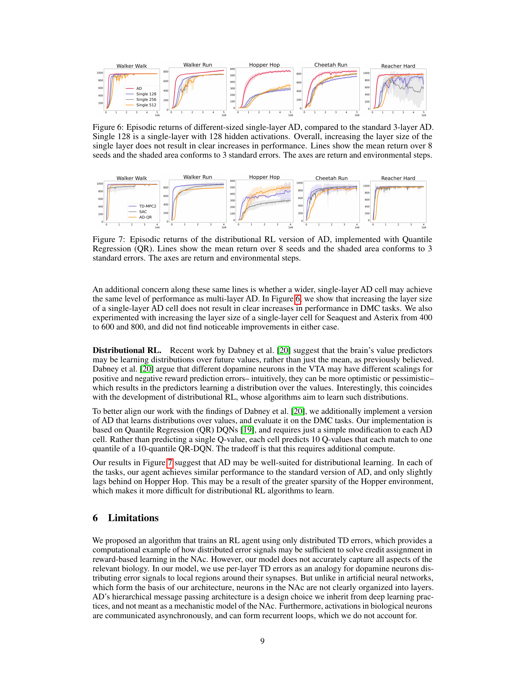
🔼 This figure shows an ablation study comparing the performance of the proposed 3-layer AD network against single-layer AD networks with different numbers of hidden units (128, 256, and 512). The results show that increasing the size of the single layer does not significantly improve performance, indicating the importance of multiple layers in the AD architecture for effective learning. The plot displays the mean episodic return for each network configuration over eight random seeds. Error bars representing 3 standard errors are also provided to show the variability in performance.
read the caption
Figure 6: Episodic returns of different-sized single-layer AD, compared to the standard 3-layer AD. Single 128 is a single-layer with 128 hidden activations. Overall, increasing the layer size of the single layer does not result in clear increases in performance. Lines show the mean return over 8 seeds and the shaded area conforms to 3 standard errors. The axes are return and environmental steps.

🔼 This figure presents a comparison of the performance of the ARTIFICIAL DOPAMINE (AD) algorithm against three other deep reinforcement learning algorithms (DQN, TD-MPC2, and SAC) across a range of tasks from the MinAtar and DeepMind Control Suite benchmark environments. The x-axis represents the number of environment steps, and the y-axis represents the average episodic return. The lines show the mean return achieved across 10 different random seeds for each algorithm and each environment, while the shaded areas represent the standard error of the mean. The results show that the AD algorithm achieves performance comparable to the other algorithms across most of the tested environments, suggesting that synchronously distributed per-layer temporal difference errors may be sufficient for learning.
read the caption
Figure 4: Episodic returns of AD in MinAtar and DMC environments, compared to DQN, TD-MPC2 and SAC. Lines show the mean return over 10 seeds and the shaded area conforms to 3 standard errors. The axes are return and environmental steps.

🔼 This figure compares the performance of the proposed Artificial Dopamine (AD) algorithm against three established deep reinforcement learning (RL) algorithms: Deep Q-Network (DQN), Soft Actor-Critic (SAC), and Temporal Difference Model Predictive Control (TD-MPC2). The comparison is conducted across a set of 14 tasks, which includes discrete tasks from the MinAtar environment (miniaturized Atari games) and continuous control tasks from the DeepMind Control Suite (DMC). The plot shows the mean episodic reward (average return per episode) obtained by each algorithm over 10 random seeds, with error bars indicating 3 standard errors. This visualization helps assess the relative performance of AD compared to the baselines across various task complexities.
read the caption
Figure 4: Episodic returns of AD in MinAtar and DMC environments, compared to DQN, TD-MPC2 and SAC. Lines show the mean return over 10 seeds and the shaded area conforms to 3 standard errors. The axes are return and environmental steps.

🔼 This figure presents the performance comparison of the proposed Artificial Dopamine (AD) algorithm against three established deep reinforcement learning algorithms: Deep Q-Network (DQN), Soft Actor-Critic (SAC), and Temporal Difference Model Predictive Control (TD-MPC2). The results are shown across a set of benchmark tasks from the MinAtar and DeepMind Control Suite (DMC) environments. For each environment, the mean episodic reward and its associated standard error across 10 independent trials are shown, allowing for a clear comparison of the algorithms’ performance. The x-axis represents the total number of environment steps taken, and the y-axis indicates the average episodic reward achieved.
read the caption
Figure 4: Episodic returns of AD in MinAtar and DMC environments, compared to DQN, TD-MPC2 and SAC. Lines show the mean return over 10 seeds and the shaded area conforms to 3 standard errors. The axes are return and environmental steps.
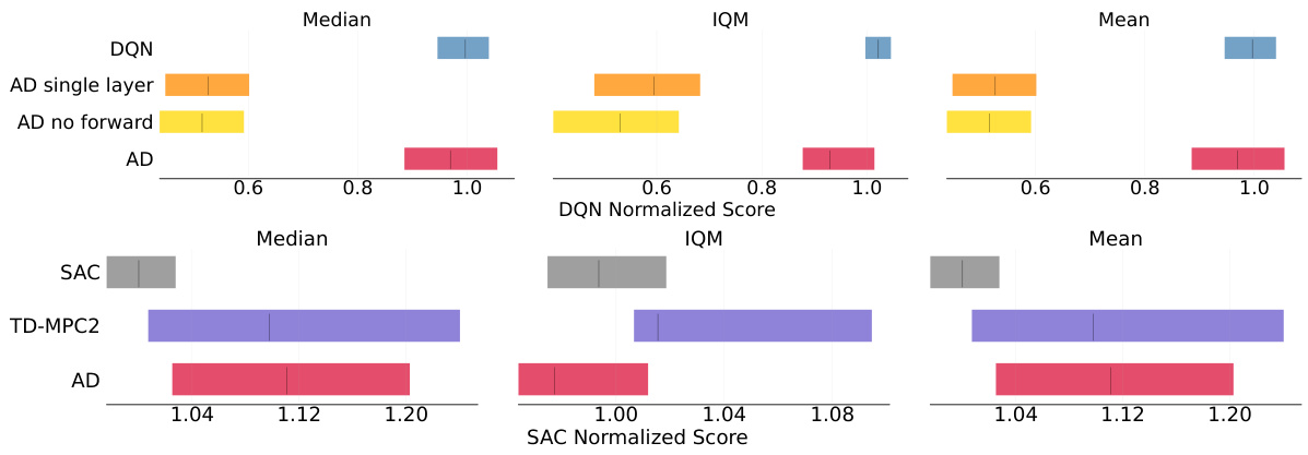
🔼 This figure compares the performance of the proposed ARTIFICIAL DOPAMINE (AD) algorithm to other state-of-the-art reinforcement learning algorithms (DQN, TD-MPC2, and SAC) across a set of 14 tasks. The tasks are split between MinAtar (discrete) and DeepMind Control Suite (DMC, continuous) environments. The x-axis represents the number of environment steps and the y-axis represents the mean episodic return. Error bars (shaded regions) represent three standard errors, indicating the variability in performance across multiple runs (10 seeds). The plot visualizes how well the AD algorithm performs compared to baselines, demonstrating comparable performance despite not using backpropagation.
read the caption
Figure 4: Episodic returns of AD in MinAtar and DMC environments, compared to DQN, TD-MPC2 and SAC. Lines show the mean return over 10 seeds and the shaded area conforms to 3 standard errors. The axes are return and environmental steps.
Full paper#
