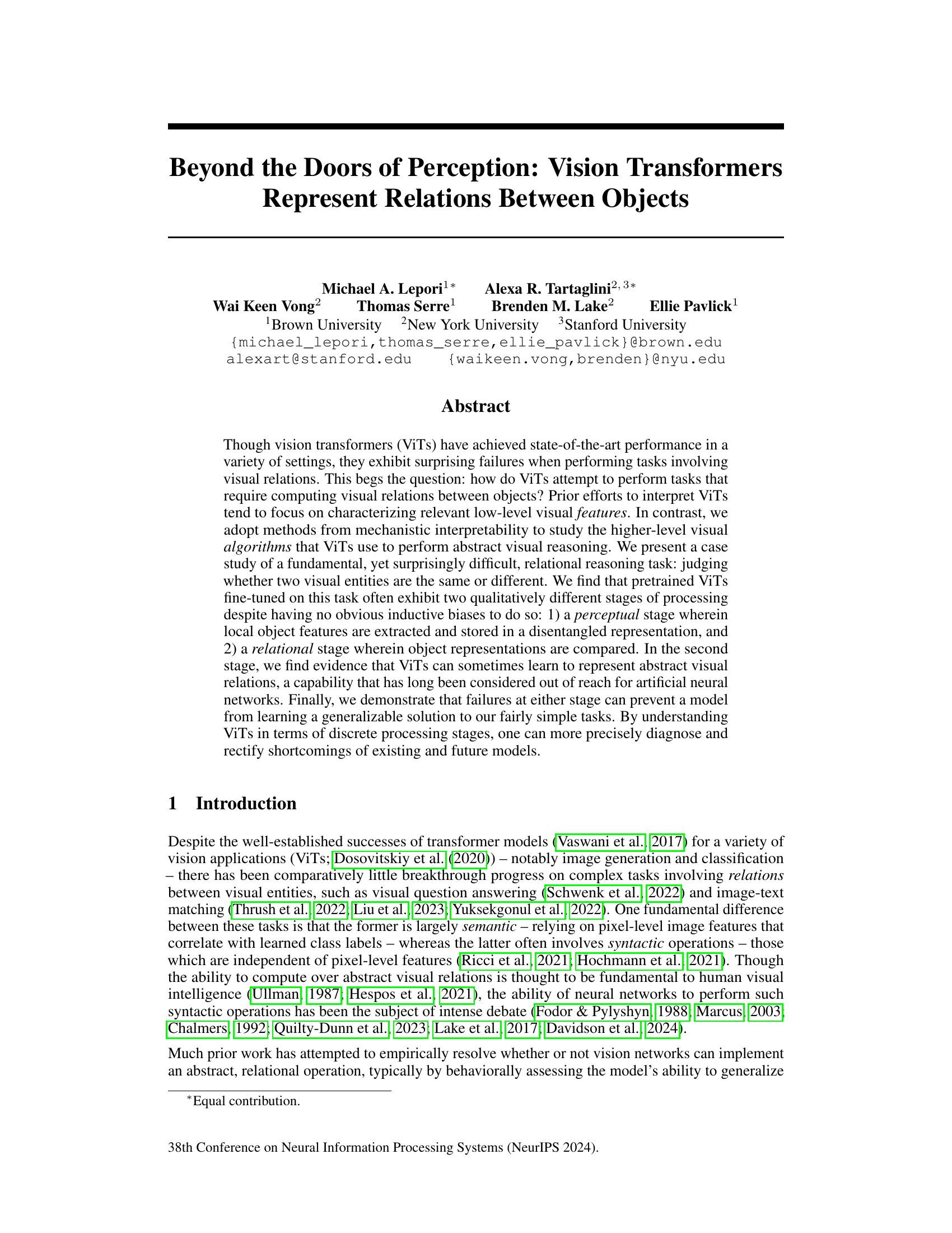
TL;DR#
Vision transformers (ViTs), while powerful in image classification and generation, surprisingly fail at tasks involving visual relations. This paper investigates why this happens by focusing on a simpler task: judging whether two visual objects are the same or different. The core problem is that existing studies focus on low-level features, neglecting higher-level visual algorithms.
The researchers used mechanistic interpretability methods to analyze pre-trained ViTs fine-tuned for this same-different task. They discovered two distinct processing stages: a perceptual stage that extracts object features and a relational stage that compares object representations. Critically, they showed that these stages must function correctly for the model to generalize to unseen stimuli. This finding contributes to the mechanistic interpretability field by clarifying the internal mechanisms of ViTs and provides valuable insights for improving their relational reasoning capabilities.
Key Takeaways#
Why does it matter?#
This paper is crucial for researchers in computer vision and cognitive science due to its novel approach in using mechanistic interpretability to understand how vision transformers (ViTs) perform relational reasoning tasks. It challenges existing assumptions about ViT capabilities and opens new avenues for improving the design and generalization of future models, especially in complex visual reasoning scenarios.
Visual Insights#
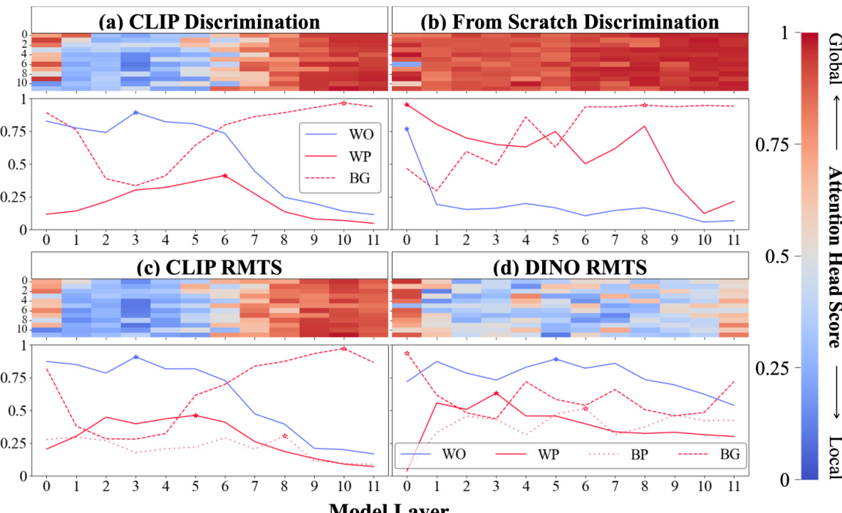
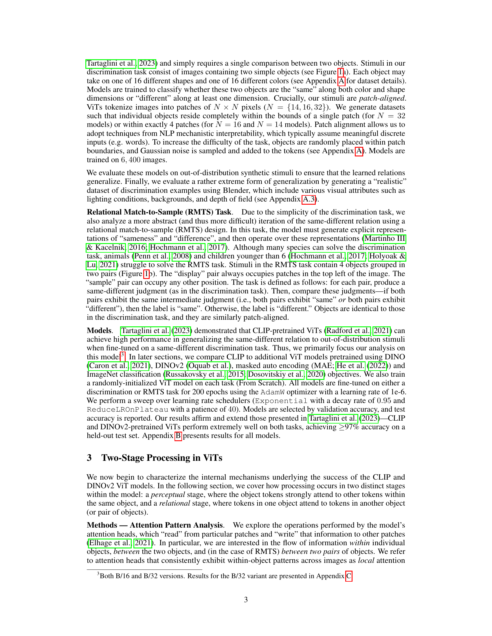
🔼 This figure visualizes the attention patterns in different ViT models trained on discrimination and RMTS tasks. It shows a transition from local (within-object) attention to global (between-object) attention, indicating a two-stage processing pipeline in some models but not others. The heatmaps depict the distribution of local and global attention heads across layers, while line graphs show the proportion of attention within an object, between objects, and in the background. The analysis reveals a hierarchical pattern in CLIP models performing the RMTS task, absent in DINO models.
read the caption
Figure 2: Attention Pattern Analysis. (a) CLIP Discrimination: The heatmap (top) shows the distribution of 'local' (blue) vs. 'global' (red) attention heads throughout a CLIP ViT-B/16 model fine-tuned on discrimination (Figure 1a). The x-axis is the model layer, while the y-axis is the head index. Local heads tend to cluster in early layers and transition to global heads around layer 6. For each layer, the line graph (bottom) plots the maximum proportion of attention across all 12 heads from object patches to image patches that are 1) within the same object (within-object=WO), 2) within the other object (within-pair=WP), or 3) in the background (BG). The stars mark the peak of each. WO attention peaks in early layers, followed by WP, and finally BG. (b) From Scratch Discrimination: We repeat the analysis in (a). The model contains nearly zero local heads. (c) CLIP RMTS: We repeat the analysis for a CLIP model fine-tuned on RMTS (Figure 1b). Top: Our results largely hold from (a). Bottom: We track a fourth attention pattern-attention between pairs of objects (between pair=BP). We find that WO peaks first, then WP, then BP, and finally BG. This accords with the hierarchical computations implied by the RMTS task. (d) DINO RMTS: We repeat the analysis in (c) for a DINO model and find no such hierarchical pattern.
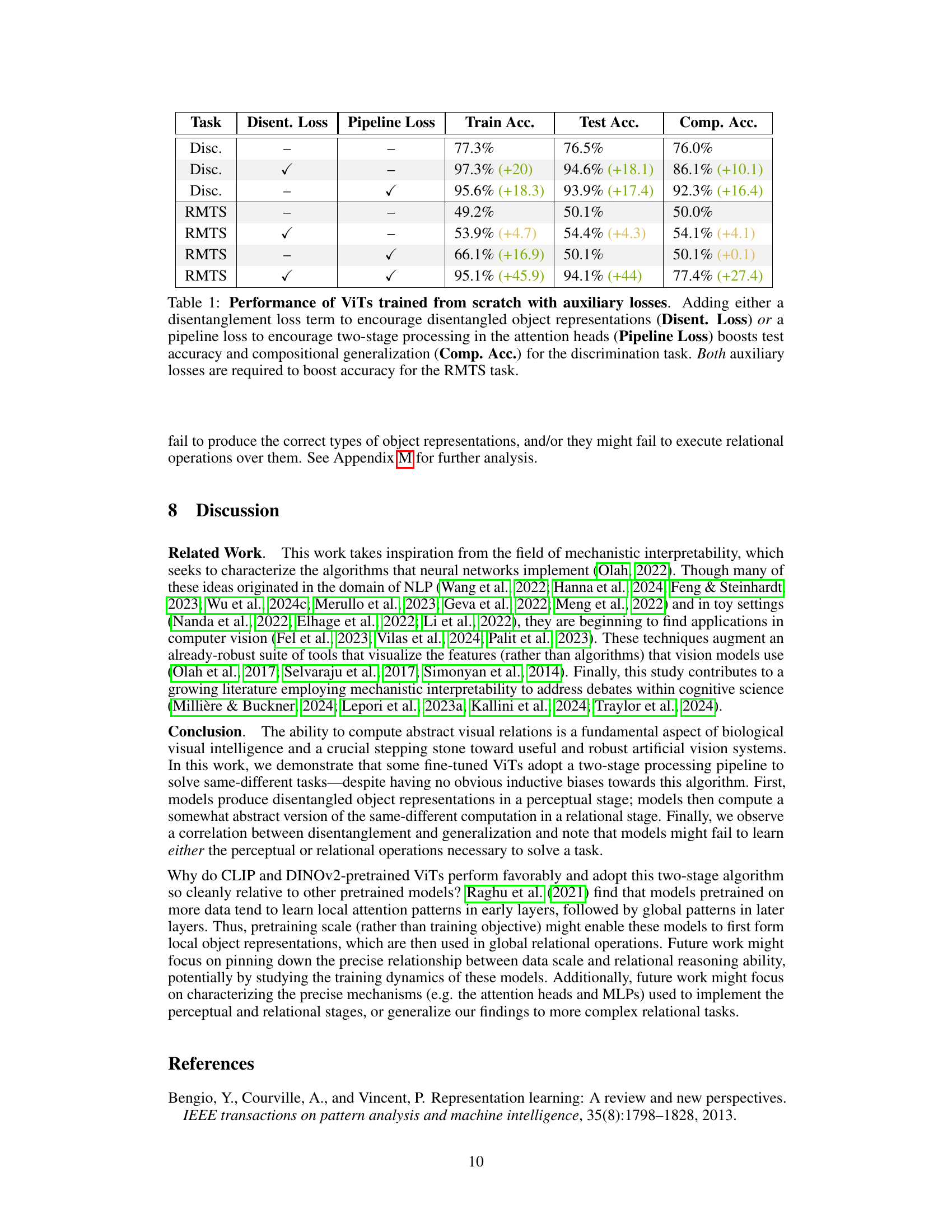
🔼 This table presents the performance of Vision Transformers (ViTs) trained from scratch on discrimination and relational match-to-sample (RMTS) tasks. It shows the impact of adding auxiliary loss functions (disentanglement loss and pipeline loss) on training accuracy, test accuracy, and compositional generalization accuracy. The results demonstrate that these losses improve performance, especially for the more complex RMTS task, highlighting the importance of disentangled representations and two-stage processing.
read the caption
Table 1: Performance of ViTs trained from scratch with auxiliary losses. Adding either a disentanglement loss term to encourage disentangled object representations (Disent. Loss) or a pipeline loss to encourage two-stage processing in the attention heads (Pipeline Loss) boosts test accuracy and compositional generalization (Comp. Acc.) for the discrimination task. Both auxiliary losses are required to boost accuracy for the RMTS task.
In-depth insights#
ViT Relational Reasoning#
The study of ViT relational reasoning explores how Vision Transformers (ViTs), despite their success in various visual tasks, surprisingly struggle with tasks involving relationships between objects. The core issue lies in ViTs’ architecture, which processes image patches independently before aggregating information. This limits their ability to directly model relationships, unlike models explicitly designed for relational reasoning. Mechanistic interpretability is employed to analyze the internal processes of ViTs, revealing a two-stage architecture. The first stage focuses on perceptual processing of individual objects, while the second stage attempts relational reasoning, comparing object representations. The researchers identify this two-stage process in some ViTs, showing that they can represent abstract visual relations. However, the study also reveals that failure in either stage (perceptual or relational) hinders accurate performance. Successful relational reasoning requires both accurate disentangled object representations (perceptual stage) and effective mechanisms for comparing these representations (relational stage). Counterfactual interventions are used to demonstrate disentanglement in the perceptual stage. Notably, the study introduces a novel synthetic relational match-to-sample task, highlighting the challenges involved in evaluating ViT’s relational capabilities. The results show a correlation between disentanglement and model generalization. Overall, the paper provides crucial insights into the limitations and potential solutions for improving ViT’s relational reasoning performance.
Two-Stage Processing#
The study’s “Two-Stage Processing” analysis reveals a compelling mechanism in Vision Transformers (ViTs). ViTs, when fine-tuned for same-different tasks, exhibit a clear division of labor: an initial perceptual stage focused on disentangling local object features (shape and color), followed by a relational stage dedicated to abstract relational comparisons. This two-stage process is not inherent to the architecture, but rather a learned behavior, as evidenced by the model’s capacity for abstract reasoning. The model’s success hinges on the integrity of both stages; failures in either perception (feature extraction) or relation (comparison) hinder accurate same-different judgments. Disentanglement of features is crucial for generalization, particularly to out-of-distribution data, highlighting the importance of developing methods to induce disentanglement in model training. This work not only unveils the internal workings of ViTs but also offers valuable insights into designing more robust and generalizable relational reasoning models.
Disentangled Features#
Disentangled features represent a crucial concept in the context of machine learning, particularly within the field of generative models and representation learning. The core idea revolves around creating a model where individual features are independent and easily manipulable; changing one feature doesn’t inadvertently affect others. This is desirable because it allows for better understanding of learned representations, facilitates easier control over the generation process, and boosts generalization capabilities to unseen data combinations. Achieving disentanglement is challenging, however, and often requires carefully designed architectures and training procedures that promote independent feature learning. Methods like Variational Autoencoders (VAEs) and Generative Adversarial Networks (GANs) have been extensively employed, but perfecting disentanglement remains an active area of research. Successful disentanglement offers several benefits such as improved interpretability and control, increased data efficiency, and enhanced robustness against variations in input features.
Relational Stage Limits#
The limitations of the relational stage in vision transformers (ViTs) represent a critical bottleneck in their ability to perform complex visual reasoning tasks. ViTs, while excelling at low-level feature extraction, often struggle to generalize relational understanding to unseen combinations or variations of objects. This inability highlights the need for more robust relational mechanisms within ViT architectures. One key aspect to explore further is the nature of the representations used in this stage; are they truly abstract, disentangled, and compositional, or do they rely on memorization of specific object configurations? Addressing this requires a deeper investigation into how ViTs learn to represent and operate over abstract visual relations and how this process can be improved through architectural innovations or training methodologies. Ultimately, the findings suggest that even relatively simple relational tasks pose significant challenges for current ViT designs, implying a necessity for future research to focus on enhancing their capabilities in this area.
Future Work Directions#
Future research should explore generalizing these findings to more complex relational reasoning tasks, extending beyond simple same-different judgments. Investigating the impact of different pretraining datasets and architectures on the emergence of two-stage processing is crucial. A deeper mechanistic analysis, potentially using techniques like circuit analysis or causal inference, could reveal the specific computations performed in each stage. Developing regularizers to explicitly promote disentanglement and two-stage processing could lead to more robust models. Furthermore, exploring the relationship between model scalability (in terms of dataset size and model parameters) and the ability to perform abstract visual relational reasoning is vital. Finally, a thorough examination of failure modes in both stages, potentially incorporating new loss functions or architectural modifications, would greatly advance our understanding of relational reasoning in vision transformers.
More visual insights#
More on figures

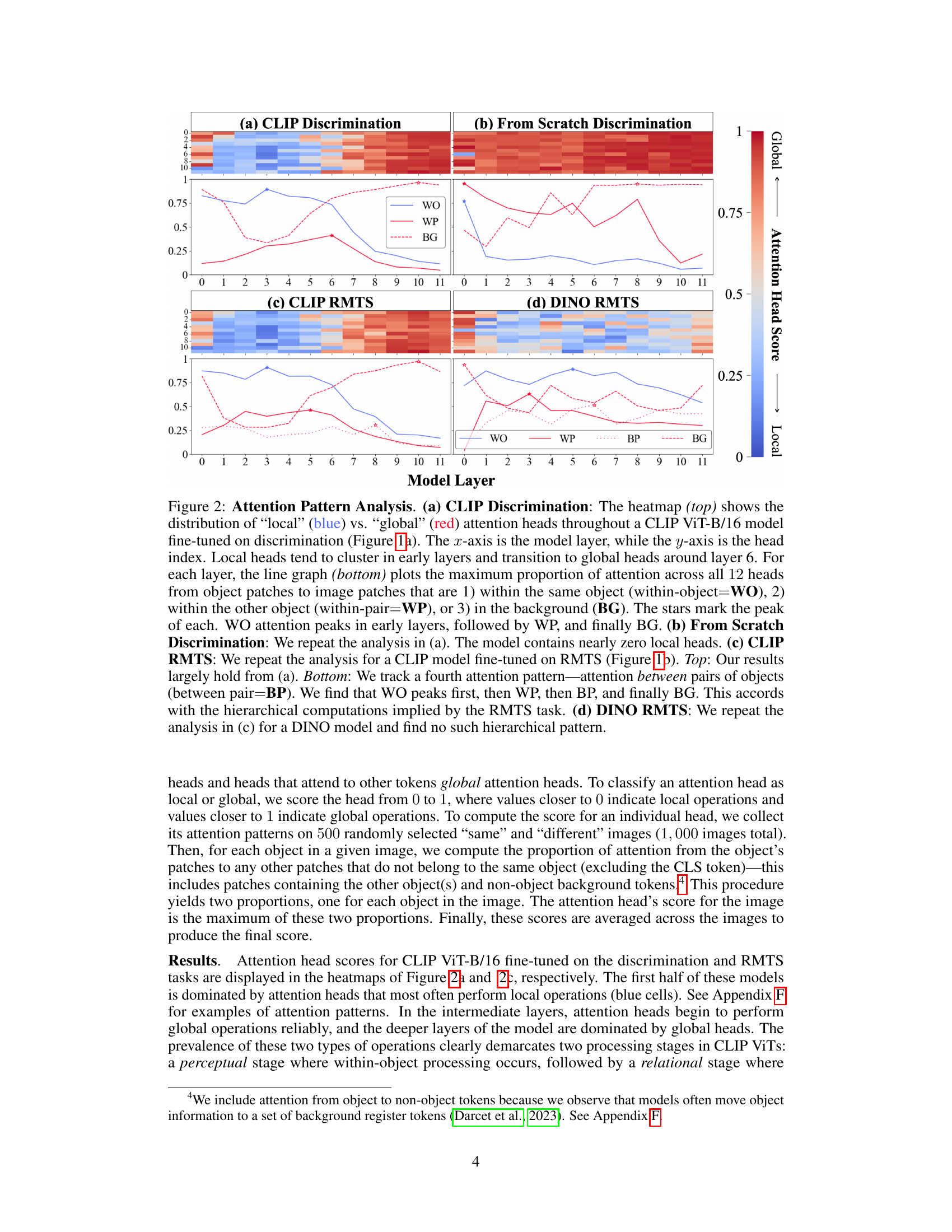
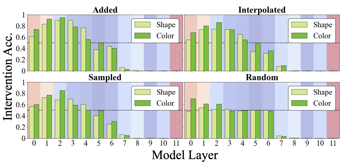
🔼 Figure 3(a) shows the method of interchange intervention used to test if the model’s shape and color features are disentangled. Figure 3(b) shows the results of applying this method to CLIP ViT-B/16 model fine-tuned on discrimination and RMTS tasks. The results indicate that shape and color are disentangled in the early layers of the model.
read the caption
Figure 3: (a) Interchange interventions: The base image exhibits the “different” relation, as the two objects differ in either shape (top) or color (bottom). An interchange intervention extracts {shape, color}information from the intermediate representations generated by the same model run on a different image (source), then patches this information from the source image into the model's intermediate representations of the base image. If successful, the intervened model will now return “same” when run on the base image. DAS is optimized to succeed at interchange interventions. (b) Disentanglement Results: We report the success of interchange interventions on shape and color across layers for CLIP ViT-B/16 fine-tuned on either the discrimination or RMTS task. We find that these properties are disentangled early in the model-one property can be manipulated without interfering with the other. The background is colored according to the heatmap in Figure 2a, where blue denotes local heads and red denotes global heads.
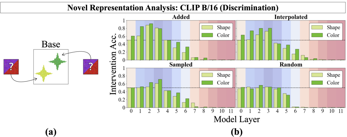
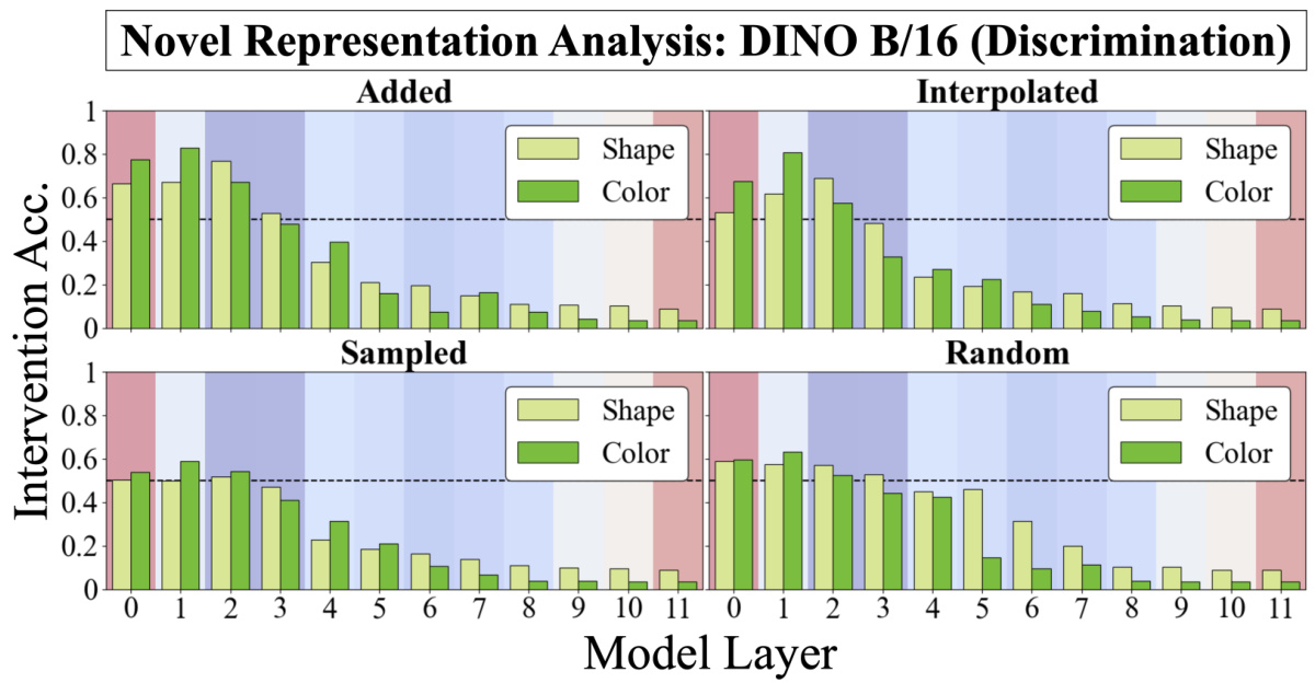
🔼 This figure shows the results of injecting novel vector representations into a CLIP model’s shape and color subspaces to assess whether the model’s same/different operation generalizes to novel inputs. The results demonstrate that the model generalizes well to vectors generated by adding or interpolating existing representations, but not to randomly sampled or simply novel vectors. This supports the idea of disentangled representations in early layers.
read the caption
Figure 4: (a) Novel Representations Analysis: Using trained DAS interventions, we can inject any vector into a model's shape or color subspaces, allowing us to test whether the same-different operation can be computed over arbitrary vectors. We intervene on a 'different' image-differing only in its color property-by patching a novel color (an interpolation of red and black) into both objects in order to flip the decision to 'same'. (b) Discrimination Results: We perform novel representations analysis using four methods for generating novel representations: 1) adding observed representations, 2) interpolating observed representations, 3) per-dimension sampling using a distribution derived from observed representations, and 4) sampling randomly from a normal distribution N(0, 1). The model's same-different operation generalizes well to vectors generated by adding (and generalizes somewhat to interpolated vectors) in early layers but not to sampled or random vectors. The background is colored according to the heatmap in Figure 2a (blue=local heads; red=global heads).

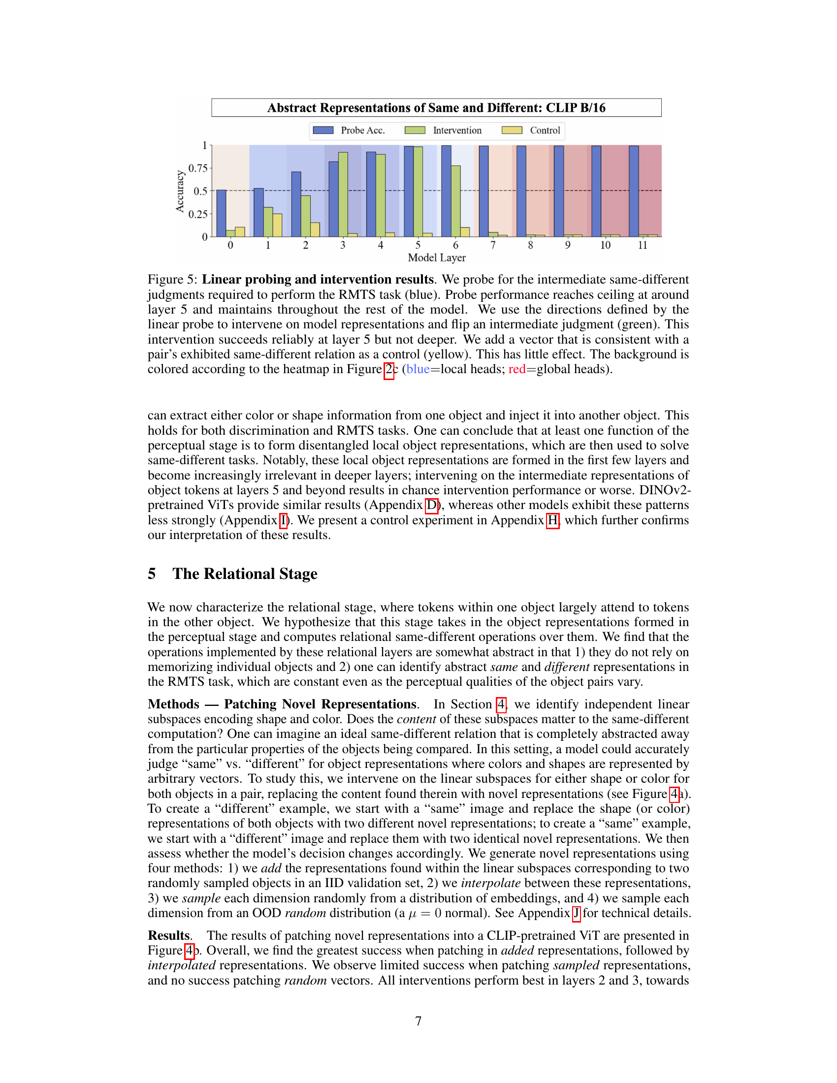
🔼 This figure shows the results of linear probing and intervention experiments designed to test the relational stage of the model. Linear probing successfully identifies the intermediate same/different judgment in layer 5, which is then used in interventions to flip a judgment. Interventions based on the probe are successful up to layer 5 but fail in deeper layers. Control interventions have little effect.
read the caption
Figure 5: Linear probing and intervention results. We probe for the intermediate same-different judgments required to perform the RMTS task (blue). Probe performance reaches ceiling at around layer 5 and maintains throughout the rest of the model. We use the directions defined by the linear probe to intervene on model representations and flip an intermediate judgment (green). This intervention succeeds reliably at layer 5 but not deeper. We add a vector that is consistent with a pair's exhibited same-different relation as a control (yellow). This has little effect. The background is colored according to the heatmap in Figure 2c (blue=local heads; red=global heads).

🔼 This figure shows the correlation between the disentanglement of object representations (measured by counterfactual intervention accuracy) and generalization performance on three different test sets: IID (in-distribution), OOD (out-of-distribution), and compositional. The results are shown for various pretrained vision transformer models (CLIP, DINO, DINOv2, ImageNet, MAE) and a model trained from scratch. The graph indicates that higher disentanglement generally leads to better generalization performance across all three test set types.
read the caption
Figure 6: We average the best counterfactual intervention accuracy for shape and color and plot it against IID, OOD, and Compositional Test set performance for CLIP, DINO, DINOv2, ImageNet, MAE, and from-scratch B/16 models. We observe that increased disentanglement (i.e. higher counterfactual accuracy) correlates with downstream performance. The from-scratch model achieved only chance IID performance in RMTS, so we omitted it from the analysis.
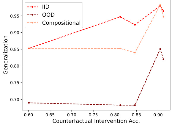
🔼 This figure shows the correlation between disentanglement (measured by counterfactual intervention accuracy) and generalization performance across different model architectures. The x-axis represents the counterfactual intervention accuracy, while the y-axis shows the generalization accuracy. Different lines represent different generalization test sets (IID, OOD, and Compositional). The results demonstrate a positive correlation: higher disentanglement leads to better generalization.
read the caption
Figure 6: We average the best counterfactual intervention accuracy for shape and color and plot it against IID, OOD, and Compositional Test set performance for CLIP, DINO, DINOv2, ImageNet, MAE, and from-scratch B/16 models. We observe that increased disentanglement (i.e. higher counterfactual accuracy) correlates with downstream performance. The from-scratch model achieved only chance IID performance in RMTS, so we omitted it from the analysis.

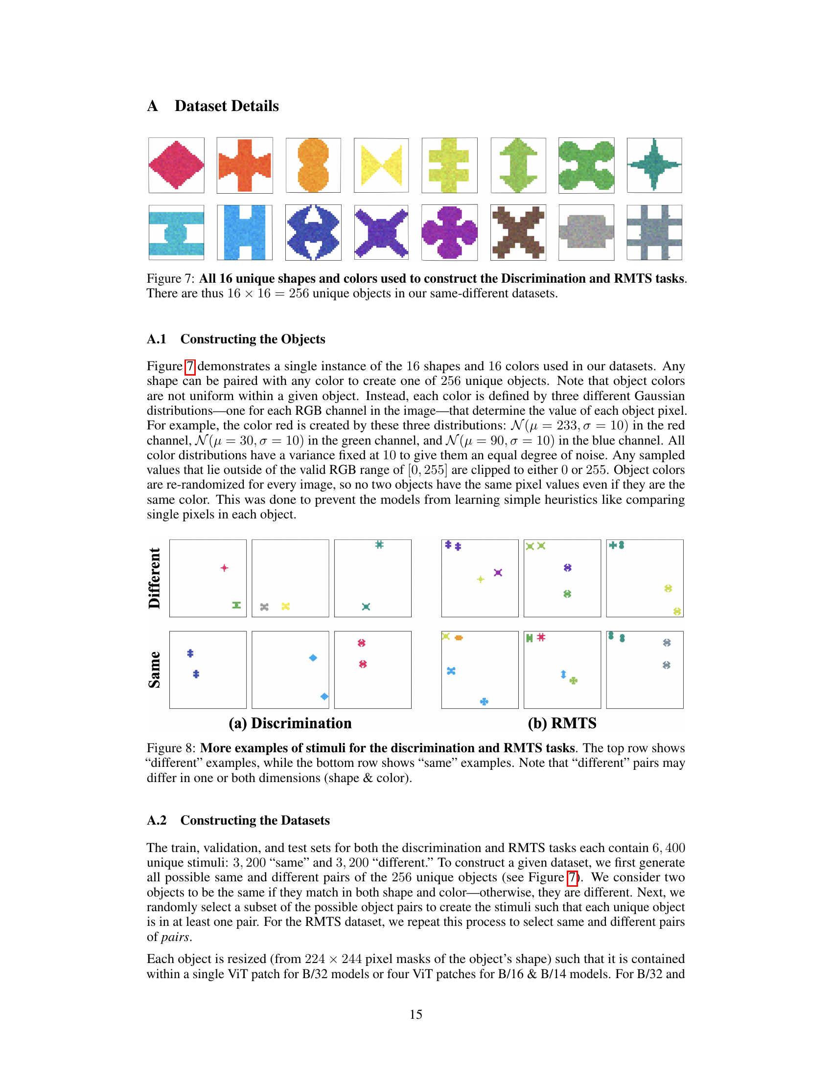
🔼 This figure shows all 16 unique shapes and 16 unique colors used to create the stimuli for the discrimination and RMTS tasks. Each shape can be combined with any color to create a unique object, resulting in a total of 256 unique objects (16 shapes * 16 colors = 256 objects). These objects form the basis of the same-different datasets used in the experiments described in the paper.
read the caption
Figure 7: All 16 unique shapes and colors used to construct the Discrimination and RMTS tasks. There are thus 16 × 16 = 256 unique objects in our same-different datasets.

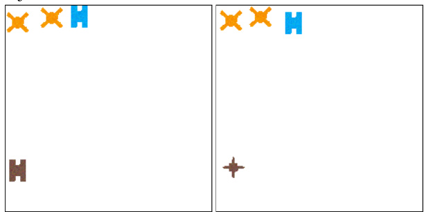
🔼 This figure shows two different tasks used to evaluate models’ ability to perform same-different judgments. The discrimination task is simple, while the Relational Match-to-Sample (RMTS) task is more complex and requires understanding abstract relations between objects.
read the caption
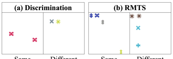
Figure 1: Two same-different tasks. (a) Discrimination: “same” images contain two objects with the same color and shape. Objects in “different” images differ in at least one of those properties—in this case, both color and shape. (b) RMTS: “same” images contain a pair of objects that exhibit the same relation as a display pair of objects in the top left corner. In the image on the left, both pairs demonstrate a “different” relation, so the classification is “same” (relation). “Different” images contain pairs exhibiting different relations.

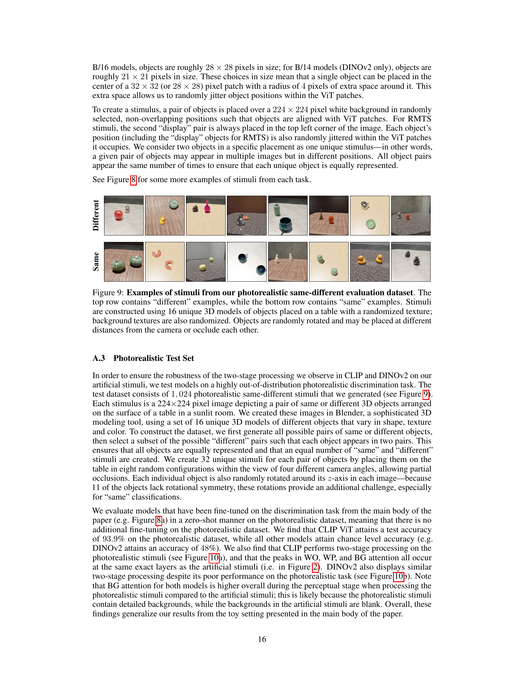
🔼 This figure shows example images from a photorealistic same-different dataset used to evaluate the robustness of the two-stage processing observed in CLIP and DINOv2 models. The top row displays pairs of objects that are different, while the bottom row shows pairs of objects that are the same. The images feature diverse 3D objects with varying textures, lighting, and object placement on a table to create a highly realistic and varied dataset.
read the caption
Figure 9: Examples of stimuli from our photorealistic same-different evaluation dataset. The top row contains “different” examples, while the bottom row contains “same” examples. Stimuli are constructed using 16 unique 3D models of objects placed on a table with a randomized texture; background textures are also randomized. Objects are randomly rotated and may be placed at different distances from the camera or occlude each other.

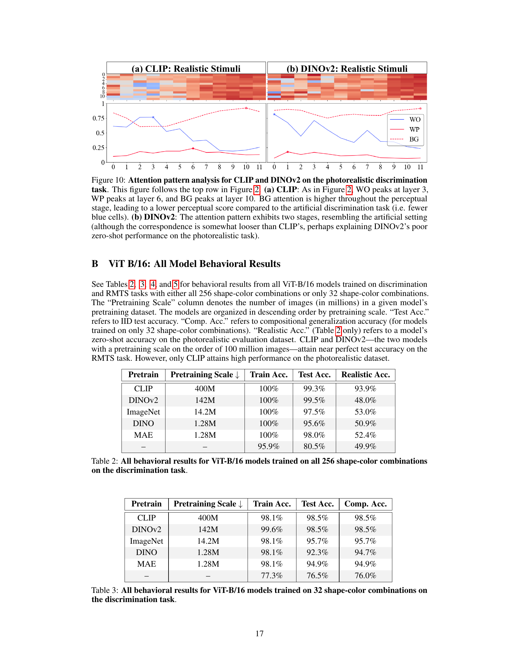
🔼 This figure shows the attention pattern analysis for CLIP and DINOv2 models on a photorealistic discrimination task. It compares the attention patterns (local vs. global) across different layers of the models. The results show that CLIP maintains a clear two-stage processing pattern (perceptual and relational) even with photorealistic images, while DINOv2’s two-stage pattern is less defined, potentially explaining its lower performance.
read the caption
Figure 10: Attention pattern analysis for CLIP and DINOv2 on the photorealistic discrimination task. This figure follows the top row in Figure 2. (a) CLIP: As in Figure 2, WO peaks at layer 3, WP peaks at layer 6, and BG peaks at layer 10. BG attention is higher throughout the perceptual stage, leading to a lower perceptual score compared to the artificial discrimination task (i.e. fewer blue cells). (b) DINOv2: The attention pattern exhibits two stages, resembling the artificial setting (although the correspondence is somewhat looser than CLIP's, perhaps explaining DINOv2's poor zero-shot performance on the photorealistic task).

🔼 This figure displays the results of an attention pattern analysis performed on four different models. It shows the distribution of ’local’ vs. ‘global’ attention heads across layers for CLIP and DINO models trained on discrimination and RMTS tasks. The analysis reveals two distinct processing stages in some models: a perceptual stage (local heads dominant, focusing within objects) and a relational stage (global heads dominant, comparing objects). The ‘From Scratch’ model shows minimal local attention heads, highlighting the role of pre-training in shaping attention patterns. DINO models do not exhibit the clear hierarchical processing observed in the CLIP models on the RMTS task.
read the caption
Figure 2: Attention Pattern Analysis. (a) CLIP Discrimination: The heatmap (top) shows the distribution of 'local' (blue) vs. 'global' (red) attention heads throughout a CLIP ViT-B/16 model fine-tuned on discrimination (Figure 1a). The x-axis is the model layer, while the y-axis is the head index. Local heads tend to cluster in early layers and transition to global heads around layer 6. For each layer, the line graph (bottom) plots the maximum proportion of attention across all 12 heads from object patches to image patches that are 1) within the same object (within-object=WO), 2) within the other object (within-pair=WP), or 3) in the background (BG). The stars mark the peak of each. WO attention peaks in early layers, followed by WP, and finally BG. (b) From Scratch Discrimination: We repeat the analysis in (a). The model contains nearly zero local heads. (c) CLIP RMTS: We repeat the analysis for a CLIP model fine-tuned on RMTS (Figure 1b). Top: Our results largely hold from (a). Bottom: We track a fourth attention pattern-attention between pairs of objects (between pair=BP). We find that WO peaks first, then WP, then BP, and finally BG. This accords with the hierarchical computations implied by the RMTS task. (d) DINO RMTS: We repeat the analysis in (c) for a DINO model and find no such hierarchical pattern.

🔼 This figure shows the results of using interchange interventions, a technique used to assess whether properties like shape and color are disentangled (separately represented) in a model’s intermediate representations. (a) Illustrates the method: properties from one image are swapped into another to see if the model’s prediction changes. (b) shows the success rate of these interventions across different layers of a CLIP ViT-B/16 model, indicating disentanglement occurs early in the processing pipeline.
read the caption
Figure 3: (a) Interchange interventions: The base image exhibits the “different” relation, as the two objects differ in either shape (top) or color (bottom). An interchange intervention extracts {shape, color}information from the intermediate representations generated by the same model run on a different image (source), then patches this information from the source image into the model's intermediate representations of the base image. If successful, the intervened model will now return “same” when run on the base image. DAS is optimized to succeed at interchange interventions. (b) Disentanglement Results: We report the success of interchange interventions on shape and color across layers for CLIP ViT-B/16 fine-tuned on either the discrimination or RMTS task. We find that these properties are disentangled early in the model—one property can be manipulated without interfering with the other. The background is colored according to the heatmap in Figure 2a, where blue denotes local heads and red denotes global heads.
🔼 This figure demonstrates the results of novel representation analysis conducted on a CLIP ViT-B/16 model fine-tuned on a discrimination task. The analysis aims to understand how the model’s same-different operation generalizes to novel, unseen vector representations of shape and color. Four methods were used to generate these novel representations: adding, interpolating, sampling from observed distributions, and sampling randomly from a normal distribution. The results, shown as intervention accuracy across model layers, reveal that the model generalizes well to added and interpolated vectors in early layers, but not to sampled or random vectors. The color-coding of the background corresponds to the heatmap in Figure 2a, indicating the distribution of local and global attention heads across model layers.
read the caption
Figure 4: (a) Novel Representations Analysis: Using trained DAS interventions, we can inject any vector into a model's shape or color subspaces, allowing us to test whether the same-different operation can be computed over arbitrary vectors. We intervene on a 'different' image-differing only in its color property-by patching a novel color (an interpolation of red and black) into both objects in order to flip the decision to 'same'. (b) Discrimination Results: We perform novel representations analysis using four methods for generating novel representations: 1) adding observed representations, 2) interpolating observed representations, 3) per-dimension sampling using a distribution derived from observed representations, and 4) sampling randomly from a normal distribution N(0, 1). The model's same-different operation generalizes well to vectors generated by adding (and generalizes somewhat to interpolated vectors) in early layers but not to sampled or random vectors. The background is colored according to the heatmap in Figure 2a (blue=local heads; red=global heads).

🔼 This figure shows the results of linear probing and intervention experiments on a CLIP-pretrained ViT model fine-tuned on the RMTS task. Linear probing was used to identify the layers responsible for the same-different judgment. Interventions involved manipulating model representations to change the judgment and a control intervention that kept the same judgment. The results show that the same-different judgment is made reliably in layer 5 but not deeper, indicating that the model uses abstract representations of same and different.
read the caption
Figure 5: Linear probing and intervention results. We probe for the intermediate same-different judgments required to perform the RMTS task (blue). Probe performance reaches ceiling at around layer 5 and maintains throughout the rest of the model. We use the directions defined by the linear probe to intervene on model representations and flip an intermediate judgment (green). This intervention succeeds reliably at layer 5 but not deeper. We add a vector that is consistent with a pair's exhibited same-different relation as a control (yellow). This has little effect. The background is colored according to the heatmap in Figure 2c (blue=local heads; red=global heads).
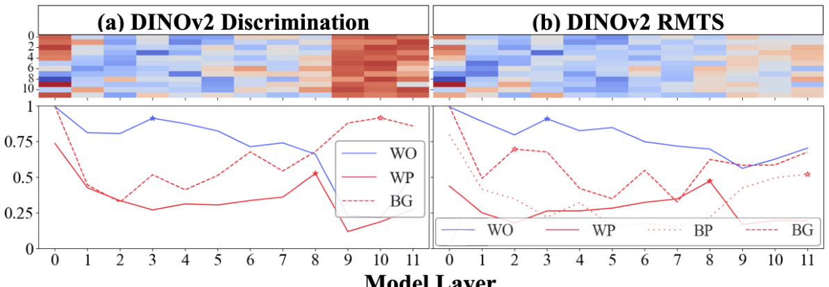
🔼 The figure shows the attention pattern analysis for DINOv2 pretrained ViTs on the discrimination and RMTS tasks. Similar to Figure 2, the heatmap shows the distribution of local and global attention heads throughout the network. The line graphs show the maximum proportion of attention from object patches to other patches that are within the same object (WO), within the other object (WP), in the background (BG), and between pairs of objects (BP for RMTS). Unlike Figure 2, the stars on the line charts mark the maximal value excluding the 0th layer because all types of attention spike in DINOv2 in the 0th layer. The results show that DINOv2 exhibits two stages of processing, similar to CLIP, but with some differences in the attention patterns.
read the caption
Figure 15: DINOv2 attention pattern analysis. See the caption of Figure 2 for figure and legend descriptions. Note that the stars in the line charts are placed differently in this figure compared to other attention pattern analysis figures. Instead of marking the maximal values of each type of attention across all 12 layers, the stars mark the maximal value excluding the 0th layer. This is because all types of attention spike in DINOv2 in the 0th layer.

🔼 This figure shows the results of applying the Distributed Alignment Search (DAS) method to a DINOv2 ViT-B/14 model. The DAS method is used to identify whether the model’s internal representations of shape and color are disentangled. The graph shows the success rate of counterfactual interventions at each layer of the model for shape and color on two tasks: a discrimination task (Disc.) and a relational match-to-sample task (RMTS). The higher the intervention accuracy, the more disentangled the representation is. The horizontal dashed line indicates chance performance.
read the caption
Figure 16: DAS results for DINOv2 ViT-B/14.
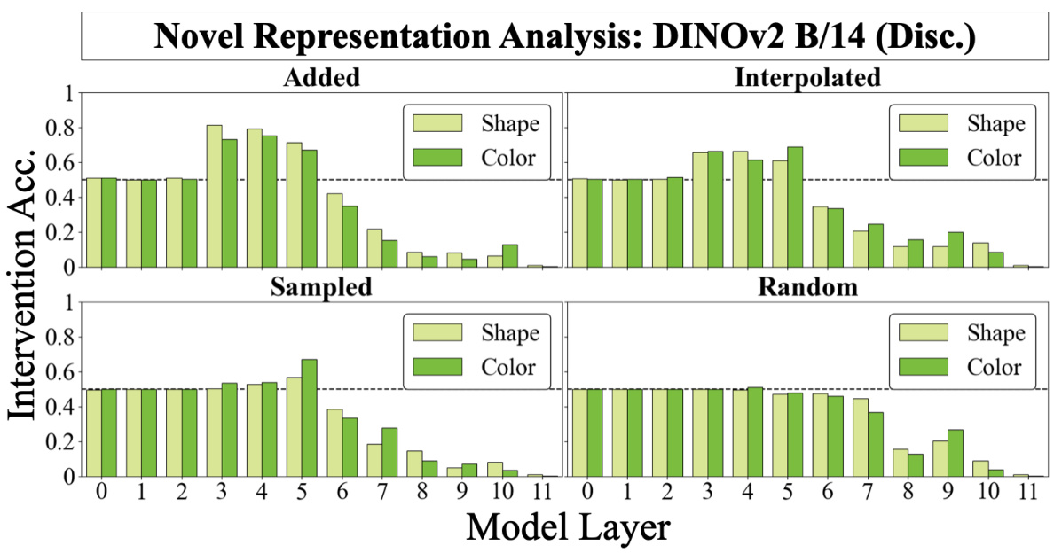
🔼 This figure shows the results of novel representation analysis for DINO ViT-B/16 model fine-tuned on the discrimination task. It uses four methods for generating novel representations: adding observed representations, interpolating observed representations, per-dimension sampling using a distribution derived from observed representations, and sampling randomly from a normal distribution. The results are shown separately for shape and color subspaces, across different model layers. The figure helps understand how well the model’s same-different operation generalizes to vectors generated by these methods.
read the caption
Figure 30: Novel Representation Analysis for DINO ViT-B/16 (Disc.).

🔼 This figure shows the attention patterns for CLIP and DINOv2 models on a photorealistic discrimination task. It demonstrates a two-stage processing pattern similar to that observed in the artificial data, with local attention (within-object) followed by global attention (between objects). However, the DINOv2 model shows a less clear separation of stages, potentially explaining its lower performance compared to CLIP.
read the caption
Figure 10: Attention pattern analysis for CLIP and DINOv2 on the photorealistic discrimination task. This figure follows the top row in Figure 2. (a) CLIP: As in Figure 2, WO peaks at layer 3, WP peaks at layer 6, and BG peaks at layer 10. BG attention is higher throughout the perceptual stage, leading to a lower perceptual score compared to the artificial discrimination task (i.e. fewer blue cells). (b) DINOv2: The attention pattern exhibits two stages, resembling the artificial setting (although the correspondence is somewhat looser than CLIP's, perhaps explaining DINOv2's poor zero-shot performance on the photorealistic task).
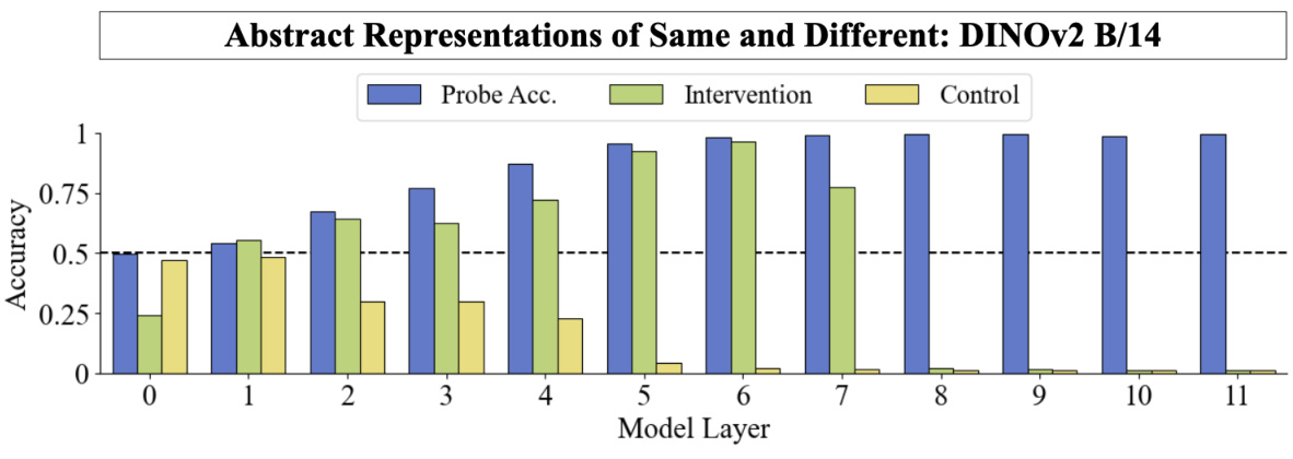
🔼 This figure shows the results of probing and intervention experiments designed to assess the relational stage of ViTs in performing the RMTS task. Linear probes identify the intermediate same-different judgments. Interventions attempt to flip the judgment by adding a vector derived from the probes. Successful interventions indicate abstract same/different representations exist in these layers, which do not solely depend on object features.
read the caption
Figure 5: Linear probing and intervention results. We probe for the intermediate same-different judgments required to perform the RMTS task (blue). Probe performance reaches ceiling at around layer 5 and maintains throughout the rest of the model. We use the directions defined by the linear probe to intervene on model representations and flip an intermediate judgment (green). This intervention succeeds reliably at layer 5 but not deeper. We add a vector that is consistent with a pair’s exhibited same-different relation as a control (yellow). This has little effect. The background is colored according to the heatmap in Figure 2c (blue=local heads; red=global heads).
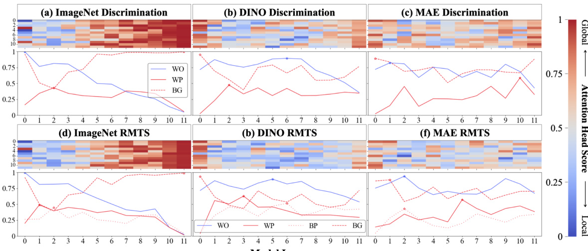
🔼 This figure analyzes attention patterns in CLIP and DINO vision transformers (ViTs) fine-tuned on discrimination and relational match-to-sample (RMTS) tasks. Heatmaps show the distribution of ’local’ and ‘global’ attention heads across model layers. Line graphs show the proportion of attention within the same object, within the other object, and in the background. The results reveal a two-stage processing pipeline (perceptual and relational) in CLIP but not in DINO, highlighting differences in how the models process these tasks.
read the caption
Figure 2: Attention Pattern Analysis. (a) CLIP Discrimination: The heatmap (top) shows the distribution of 'local' (blue) vs. 'global' (red) attention heads throughout a CLIP ViT-B/16 model fine-tuned on discrimination (Figure 1a). The x-axis is the model layer, while the y-axis is the head index. Local heads tend to cluster in early layers and transition to global heads around layer 6. For each layer, the line graph (bottom) plots the maximum proportion of attention across all 12 heads from object patches to image patches that are 1) within the same object (within-object=WO), 2) within the other object (within-pair=WP), or 3) in the background (BG). The stars mark the peak of each. WO attention peaks in early layers, followed by WP, and finally BG. (b) From Scratch Discrimination: We repeat the analysis in (a). The model contains nearly zero local heads. (c) CLIP RMTS: We repeat the analysis for a CLIP model fine-tuned on RMTS (Figure 1b). Top: Our results largely hold from (a). Bottom: We track a fourth attention pattern-attention between pairs of objects (between pair=BP). We find that WO peaks first, then WP, then BP, and finally BG. This accords with the hierarchical computations implied by the RMTS task. (d) DINO RMTS: We repeat the analysis in (c) for a DINO model and find no such hierarchical pattern.

🔼 This figure analyzes attention patterns in CLIP and DINO Vision Transformers (ViTs) fine-tuned on discrimination and relational match-to-sample (RMTS) tasks. It shows the distribution of local vs. global attention heads across layers and highlights a two-stage processing pipeline (perceptual and relational stages) in CLIP but not in DINO. The RMTS task reveals a hierarchical attention pattern in CLIP, reflecting the task’s structure.
read the caption
Figure 2: Attention Pattern Analysis. (a) CLIP Discrimination: The heatmap (top) shows the distribution of 'local' (blue) vs. 'global' (red) attention heads throughout a CLIP ViT-B/16 model fine-tuned on discrimination (Figure 1a). The x-axis is the model layer, while the y-axis is the head index. Local heads tend to cluster in early layers and transition to global heads around layer 6. For each layer, the line graph (bottom) plots the maximum proportion of attention across all 12 heads from object patches to image patches that are 1) within the same object (within-object=WO), 2) within the other object (within-pair=WP), or 3) in the background (BG). The stars mark the peak of each. WO attention peaks in early layers, followed by WP, and finally BG. (b) From Scratch Discrimination: We repeat the analysis in (a). The model contains nearly zero local heads. (c) CLIP RMTS: We repeat the analysis for a CLIP model fine-tuned on RMTS (Figure 1b). Top: Our results largely hold from (a). Bottom: We track a fourth attention pattern-attention between pairs of objects (between pair=BP). We find that WO peaks first, then WP, then BP, and finally BG. This accords with the hierarchical computations implied by the RMTS task. (d) DINO RMTS: We repeat the analysis in (c) for a DINO model and find no such hierarchical pattern.

🔼 This figure shows how CLIP processes an image to solve the discrimination task. It shows the different stages of processing, from tokenization to the final classification decision. The figure highlights the different attention patterns used at each stage, showing how the model moves from local to global processing.
read the caption
Figure 22: How CLIP ViT-B/16 processes an example from the discrimination task. Four attention heads are randomly selected from different stages in CLIP and analyzed on a single input image (see Figure 21). 1. Embedding: The model first tokenizes the input image. Each object occupies four ViT patches. 2. Layer 1, Head 5: During the perceptual stage, the model first performs low-level visual operations between tokens of individual objects. This particular attention head performs left-to-right attention within objects. 3. Layer 5, Head 9: Near the end of the perceptual stage, whole-object representations have been formed. 4. Layer 6, Head 11: During the relational stage, the whole-object representations are compared. 5. Layer 10, Head 6: Object and background tokens are used as registers to store information—presumably the classification.

🔼 This figure shows two examples of same-different tasks used in the paper. The first is a simple discrimination task where the model must determine if two objects have the same color and shape. The second is a more complex relational match-to-sample (RMTS) task, where the model must identify if two pairs of objects share the same relationship.
read the caption
Figure 1: Two same-different tasks. (a) Discrimination: “same” images contain two objects with the same color and shape. Objects in “different” images differ in at least one of those properties—in this case, both color and shape. (b) RMTS: “same” images contain a pair of objects that exhibit the same relation as a display pair of objects in the top left corner. In the image on the left, both pairs demonstrate a “different” relation, so the classification is “same” (relation). “Different” images contain pairs exhibiting different relations.
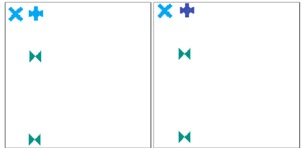
🔼 This figure shows more examples of the stimuli used in the discrimination and relational match-to-sample (RMTS) tasks. The top row displays pairs of objects that are different (differing in either shape, color, or both), and the bottom row illustrates pairs of objects that are the same (identical in shape and color). This visually clarifies the task differences and variations in the stimuli.
read the caption
Figure 8: More examples of stimuli for the discrimination and RMTS tasks. The top row shows “different” examples, while the bottom row shows “same” examples. Note that “different” pairs may differ in one or both dimensions (shape & color).
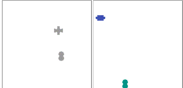
🔼 This figure shows examples of the stimuli used in the discrimination and relational match-to-sample (RMTS) tasks. The top row displays pairs of objects that are different, either in shape, color, or both. The bottom row depicts pairs of objects deemed ‘same’. This highlights the complexity of the tasks, as the definition of ‘same’ and ‘different’ can depend on multiple visual features.
read the caption
Figure 8: More examples of stimuli for the discrimination and RMTS tasks. The top row shows “different” examples, while the bottom row shows “same” examples. Note that “different” pairs may differ in one or both dimensions (shape & color).
🔼 This figure shows two example tasks used to test the models’ ability to perform same-different judgments. The first task (Discrimination) involves a simple comparison of two objects to assess whether they are the same or different in terms of shape and color. The second task (RMTS) is more complex, requiring the model to establish an abstract representation of the same-different relation between two pairs of objects. The model’s success on this second task indicates an ability to perform abstract visual reasoning.
read the caption
Figure 1: Two same-different tasks. (a) Discrimination: “same” images contain two objects with the same color and shape. Objects in “different” images differ in at least one of those properties—in this case, both color and shape. (b) RMTS: “same” images contain a pair of objects that exhibit the same relation as a display pair of objects in the top left corner. In the image on the left, both pairs demonstrate a “different” relation, so the classification is “same” (relation). “Different” images contain pairs exhibiting different relations.

🔼 The figure shows the results of two types of experiments to investigate the disentanglement of shape and color representations in the CLIP ViT-B/16 model. (a) shows the results of interchange interventions, where information from one image is swapped into another to assess the disentanglement. (b) shows the success rate of these interventions across different layers of the model, providing evidence for disentanglement. This suggests that the model learns separate representations for shape and color, which are used in later stages for higher-level relational reasoning.
read the caption
Figure 3: (a) Interchange interventions: The base image exhibits the “different” relation, as the two objects differ in either shape (top) or color (bottom). An interchange intervention extracts {shape, color}information from the intermediate representations generated by the same model run on a different image (source), then patches this information from the source image into the model's intermediate representations of the base image. If successful, the intervened model will now return “same” when run on the base image. DAS is optimized to succeed at interchange interventions. (b) Disentanglement Results: We report the success of interchange interventions on shape and color across layers for CLIP ViT-B/16 fine-tuned on either the discrimination or RMTS task. We find that these properties are disentangled early in the model-one property can be manipulated without interfering with the other. The background is colored according to the heatmap in Figure 2a, where blue denotes local heads and red denotes global heads.
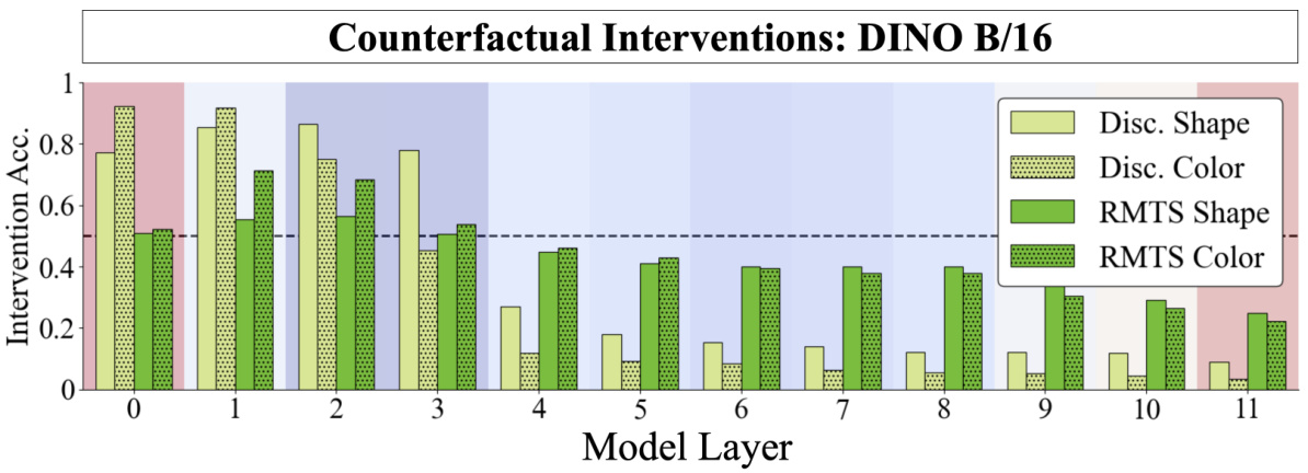
🔼 This figure shows the correlation between disentanglement and generalization performance across different ViT models. The x-axis represents the counterfactual intervention accuracy, which measures the level of disentanglement in object representations (higher values indicate better disentanglement). The y-axis shows the model’s performance on three different test sets: IID (in-distribution), OOD (out-of-distribution), and Compositional. The results show a positive correlation: models with higher disentanglement tend to perform better across all three test sets. The from-scratch model is excluded from the RMTS (Relational Match-to-Sample) analysis due to its chance-level IID performance.
read the caption
Figure 6: We average the best counterfactual intervention accuracy for shape and color and plot it against IID, OOD, and Compositional Test set performance for CLIP, DINO, DINOv2, ImageNet, MAE, and from-scratch B/16 models. We observe that increased disentanglement (i.e. higher counterfactual accuracy) correlates with downstream performance. The from-scratch model achieved only chance IID performance in RMTS, so we omitted it from the analysis.

🔼 This figure shows the correlation between disentanglement and generalization performance in different vision transformer models. Disentanglement is measured by the success rate of counterfactual interventions, which manipulate the model’s internal representations of shape and color. Generalization performance is evaluated on three test sets: IID (in-distribution), OOD (out-of-distribution), and compositional. The results indicate that higher disentanglement (better counterfactual intervention success) leads to better generalization performance across all three test sets.
read the caption
Figure 6: We average the best counterfactual intervention accuracy for shape and color and plot it against IID, OOD, and Compositional Test set performance for CLIP, DINO, DINOv2, ImageNet, MAE, and from-scratch B/16 models. We observe that increased disentanglement (i.e. higher counterfactual accuracy) correlates with downstream performance. The from-scratch model achieved only chance IID performance in RMTS, so we omitted it from the analysis.
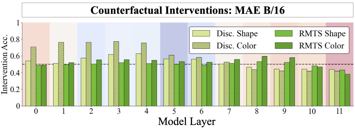
🔼 This figure shows the correlation between disentanglement (measured by counterfactual intervention accuracy) and generalization performance (on IID, OOD, and compositional test sets) across various vision transformer models. It demonstrates that models with higher disentanglement tend to generalize better. The from-scratch model, which didn’t show disentanglement, is excluded from the RMTS analysis due to poor performance.
read the caption
Figure 6: We average the best counterfactual intervention accuracy for shape and color and plot it against IID, OOD, and Compositional Test set performance for CLIP, DINO, DINOv2, ImageNet, MAE, and from-scratch B/16 models. We observe that increased disentanglement (i.e. higher counterfactual accuracy) correlates with downstream performance. The from-scratch model achieved only chance IID performance in RMTS, so we omitted it from the analysis.

🔼 This figure analyzes attention patterns in CLIP and DINO models fine-tuned on discrimination and RMTS tasks. It shows a transition from local to global attention heads across layers, indicating two processing stages: a perceptual stage (local attention, early layers) and a relational stage (global attention, later layers). The differences highlight how different model architectures approach these tasks.
read the caption
Figure 2: Attention Pattern Analysis. (a) CLIP Discrimination: The heatmap (top) shows the distribution of 'local' (blue) vs. 'global' (red) attention heads throughout a CLIP ViT-B/16 model fine-tuned on discrimination (Figure 1a). The x-axis is the model layer, while the y-axis is the head index. Local heads tend to cluster in early layers and transition to global heads around layer 6. For each layer, the line graph (bottom) plots the maximum proportion of attention across all 12 heads from object patches to image patches that are 1) within the same object (within-object=WO), 2) within the other object (within-pair=WP), or 3) in the background (BG). The stars mark the peak of each. WO attention peaks in early layers, followed by WP, and finally BG. (b) From Scratch Discrimination: We repeat the analysis in (a). The model contains nearly zero local heads. (c) CLIP RMTS: We repeat the analysis for a CLIP model fine-tuned on RMTS (Figure 1b). Top: Our results largely hold from (a). Bottom: We track a fourth attention pattern-attention between pairs of objects (between pair=BP). We find that WO peaks first, then WP, then BP, and finally BG. This accords with the hierarchical computations implied by the RMTS task. (d) DINO RMTS: We repeat the analysis in (c) for a DINO model and find no such hierarchical pattern.

🔼 This figure shows the results of novel representation analysis for CLIP ViT-B/16 on the RMTS task. It demonstrates how well the model’s same/different operation generalizes to novel object representations generated by adding, interpolating, sampling, and randomly generating vectors in the color and shape subspaces of the model. The results show that the model generalizes well to vectors generated by adding and interpolating representations in early layers, but not to sampled or random vectors. This suggests that the model has learned to represent abstract visual relations, but these representations are not completely independent of the object’s features.
read the caption
Figure 29: Novel Representation Analysis for CLIP ViT-B/16 (RMTS).
🔼 This figure shows the results of novel representation analysis for the DINO ViT-B/16 model trained on the discrimination task. It displays the intervention accuracy for each of the four methods used to generate novel representations (added, interpolated, sampled, and random) across different model layers, broken down by whether the intervention targeted the shape or color subspace. The results indicate how well the model’s same-different operation generalizes to vectors generated by these methods, providing insights into the nature of object representations learned by the model during the perceptual stage.
read the caption
Figure 30: Novel Representation Analysis for DINO ViT-B/16 (Disc.).

🔼 This figure shows the results of novel representation analysis for DINO ViT-B/16 model fine-tuned on the relational match-to-sample (RMTS) task. The analysis involved injecting novel vectors into the shape and color subspaces identified using distributed alignment search (DAS). Four methods were used to generate novel representations: adding observed representations, interpolating observed representations, per-dimension sampling using a distribution derived from observed representations, and sampling randomly from a normal distribution. The results are displayed as intervention accuracy across model layers, showing the model’s ability to generalize same/different judgments to these novel representations. The x-axis represents model layers and the y-axis represents intervention accuracy. Separate bars are shown for shape and color interventions.
read the caption
Figure 31: Novel Representation Analysis for DINO ViT-B/16 (RMTS).
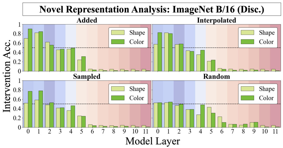
🔼 This figure shows the results of novel representation analysis on DINO ViT-B/16, fine-tuned on the discrimination task. Similar to Figure 4, it shows the success rate of interventions across different model layers, using four different methods for generating novel representations (added, interpolated, sampled, random). The results are broken down for shape and color properties separately. The figure helps assess whether the same-different operation in DINO generalizes to novel or altered vector representations of objects. The color scheme (blue to red) reflects the transition from local to global processing, observed in the model.
read the caption
Figure 30: Novel Representation Analysis for DINO ViT-B/16 (Disc.).
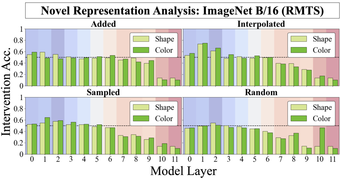
🔼 This figure displays the results of the novel representation analysis for the ImageNet ViT-B/16 model, specifically focusing on the relational match-to-sample (RMTS) task. It shows the intervention accuracy for different methods of generating novel representations (added, interpolated, sampled, random) across various model layers. The accuracy is shown separately for shape and color, demonstrating the model’s ability to generalize its ‘same’ or ‘different’ judgment to new, unseen representations. The results indicate how well the model’s internal representations have abstracted the concept of same/different away from specific visual features.
read the caption
Figure 33: Novel Representation Analysis for ImageNet ViT-B/16 (RMTS).

🔼 This figure shows the results of novel representation analysis for DINO ViT-B/16 model trained on the discrimination task. It displays the intervention accuracy for four methods of generating novel representations (adding, interpolating, sampling from observed representations, and sampling randomly) across different model layers. The results are broken down by shape and color, revealing how well the model generalizes its same-different operation to vectors that are not directly observed during training.
read the caption
Figure 30: Novel Representation Analysis for DINO ViT-B/16 (Disc.).
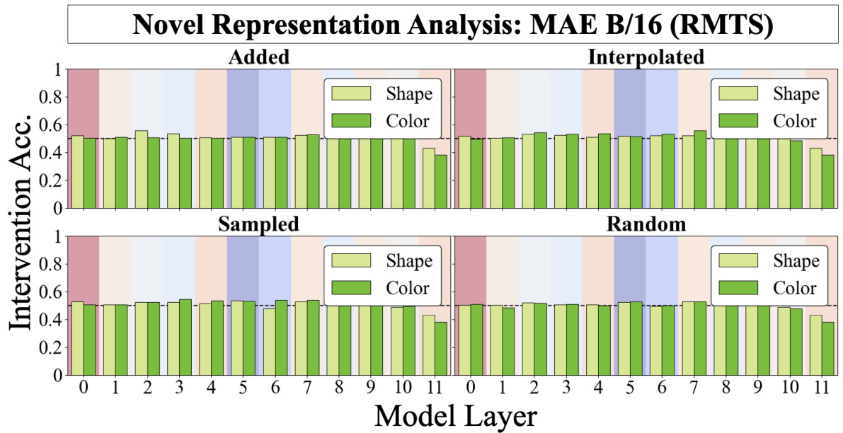
🔼 This figure shows the results of novel representation analysis for MAE ViT-B/16 model trained on RMTS task. The analysis involves injecting novel vectors into shape and color subspaces and assessing the model’s ability to perform same-different operations. The four methods of generating novel representations (adding, interpolating, sampling, and random) are displayed along with their intervention accuracy across different model layers.
read the caption
Figure 35: Novel Representation Analysis for MAE ViT-B/16 (RMTS).

🔼 The figure presents the attention pattern analysis for different models trained on two same-different tasks: discrimination and RMTS. The heatmaps show the distribution of local and global attention heads across model layers. The line graphs illustrate the maximum proportion of attention from object patches to image patches within the same object, the other object, or the background, revealing the processing stages. CLIP models exhibit a clear two-stage processing, whereas from-scratch and DINO models do not.
read the caption
Figure 2: Attention Pattern Analysis. (a) CLIP Discrimination: The heatmap (top) shows the distribution of 'local' (blue) vs. 'global' (red) attention heads throughout a CLIP ViT-B/16 model fine-tuned on discrimination (Figure 1a). The x-axis is the model layer, while the y-axis is the head index. Local heads tend to cluster in early layers and transition to global heads around layer 6. For each layer, the line graph (bottom) plots the maximum proportion of attention across all 12 heads from object patches to image patches that are 1) within the same object (within-object=WO), 2) within the other object (within-pair=WP), or 3) in the background (BG). The stars mark the peak of each. WO attention peaks in early layers, followed by WP, and finally BG. (b) From Scratch Discrimination: We repeat the analysis in (a). The model contains nearly zero local heads. (c) CLIP RMTS: We repeat the analysis for a CLIP model fine-tuned on RMTS (Figure 1b). Top: Our results largely hold from (a). Bottom: We track a fourth attention pattern-attention between pairs of objects (between pair=BP). We find that WO peaks first, then WP, then BP, and finally BG. This accords with the hierarchical computations implied by the RMTS task. (d) DINO RMTS: We repeat the analysis in (c) for a DINO model and find no such hierarchical pattern.
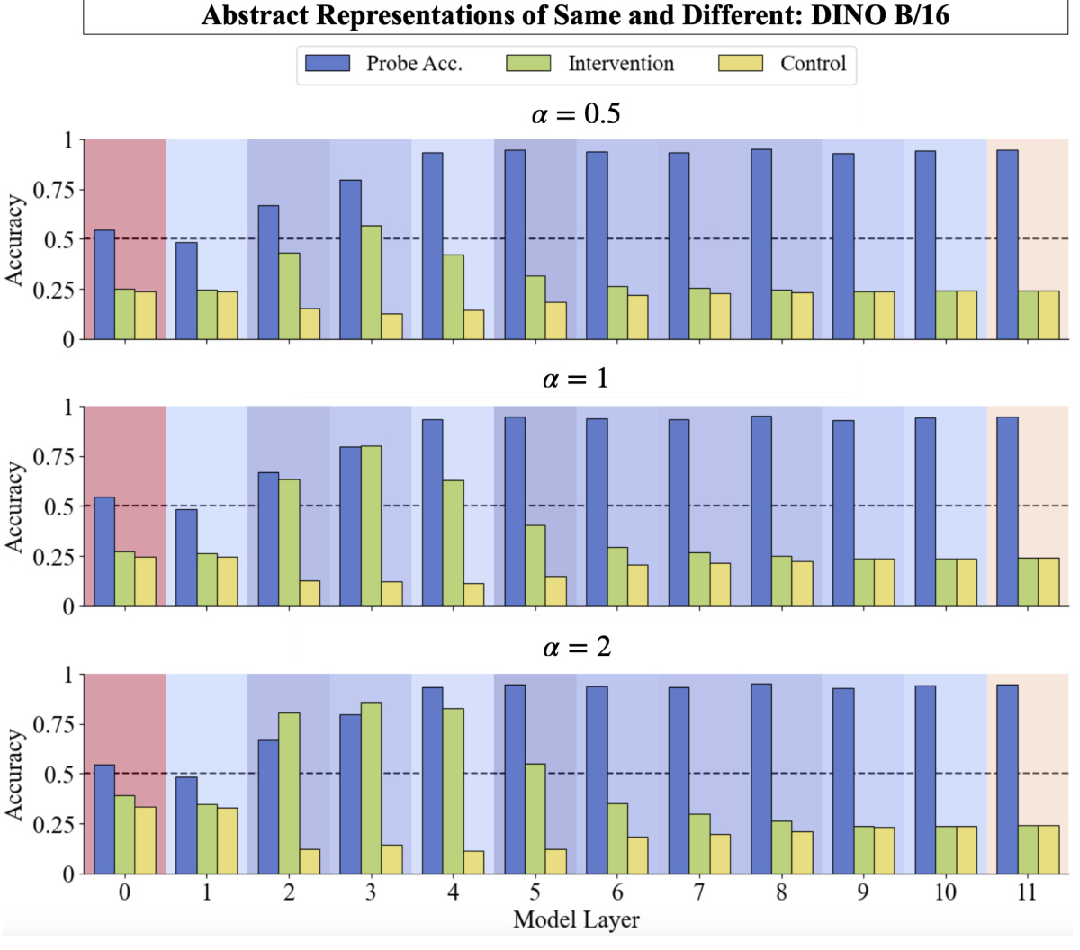
🔼 This figure displays the results of linear probing and intervention experiments performed on a DINO ViT-B/16 model. Linear probing was used to identify directions in the model’s intermediate representations that correspond to ‘same’ and ‘different’ judgments. Interventions were then performed by adding these identified directions (scaled by different factors: α = 0.5, α = 1, α = 2) to the representations. The results show the success rate of these interventions, in comparison to control interventions where unrelated vectors are added, across different layers of the model. The figure illustrates whether the model’s same-different judgment can be manipulated by adding the vectors identified by linear probing, providing insights into the model’s internal mechanisms for performing relational reasoning.
read the caption
Figure 37: Scaled linear probe & intervention analysis for DINO ViT-B/16.

🔼 This figure shows the results of linear probing and intervention experiments on a DINO ViT-B/16 model. Linear probes are used to identify intermediate same-different judgments required to perform the RMTS task, and interventions are used to flip these judgments. The results are shown for three different scaling factors (α = 0.5, 1, 2), and for each scaling factor, the results are broken down by model layer. This analysis helps to understand the extent to which intermediate representations can be used to solve more complex visual relational reasoning tasks.
read the caption
Figure 37: Scaled linear probe & intervention analysis for DINO ViT-B/16.

🔼 This figure shows the results of linear probing and intervention analysis for a MAE ViT-B/16 model on the same-different task. Linear probing is used to identify the layers where the model represents the ‘same’ and ‘different’ concepts. Interventions test whether manipulating those representations affects model decisions. The control interventions serve as a comparison.
read the caption
Figure 39: Linear probe & intervention analysis for MAE ViT-B/16.
More on tables

🔼 This table shows the performance of Vision Transformers (ViTs) trained from scratch on discrimination and relational match-to-sample (RMTS) tasks, with and without auxiliary loss functions. It demonstrates how adding disentanglement loss and/or pipeline loss improves performance, particularly on the more complex RMTS task, highlighting the benefit of disentangled representations and the two-stage processing pipeline in solving relational reasoning problems.
read the caption
Table 1: Performance of ViTs trained from scratch with auxiliary losses. Adding either a disentanglement loss term to encourage disentangled object representations (Disent. Loss) or a pipeline loss to encourage two-stage processing in the attention heads (Pipeline Loss) boosts test accuracy and compositional generalization (Comp. Acc.) for the discrimination task. Both auxiliary losses are required to boost accuracy for the RMTS task.

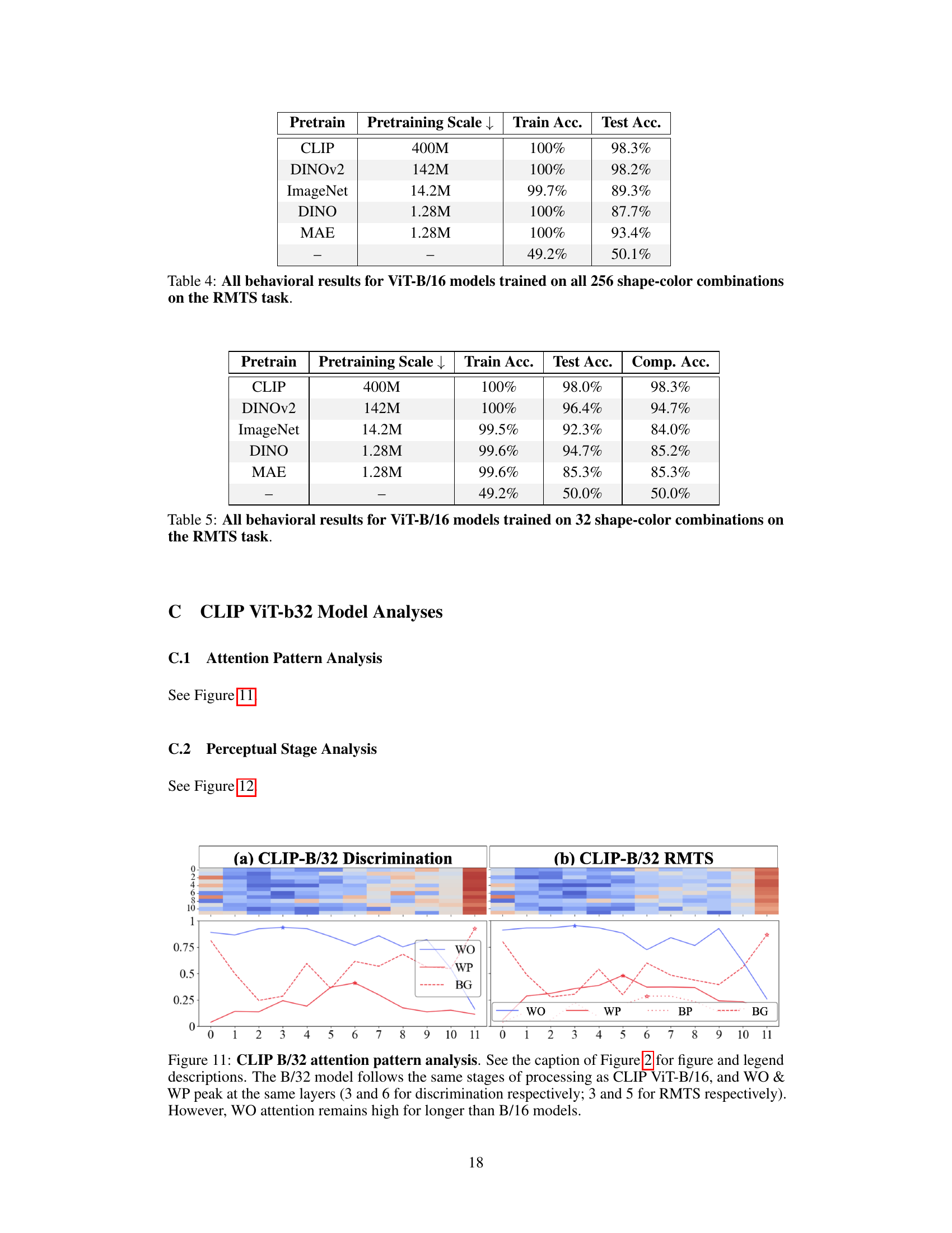
🔼 This table shows the performance of different Vision Transformer (ViT) models on a discrimination task. The models were pre-trained on different datasets (CLIP, DINOv2, ImageNet, DINO, MAE) and then fine-tuned on a discrimination task using 256 shape-color combinations. The table presents the training accuracy, test accuracy (on an IID test set), and realistic accuracy (on a photorealistic held-out test set). The results highlight the performance differences across various pre-trained ViTs, showing that CLIP and DINOv2 pretrained models generally have higher accuracy than others.
read the caption
Table 2: All behavioral results for ViT-B/16 models trained on all 256 shape-color combinations on the discrimination task.

🔼 This table presents the performance of Vision Transformers (ViTs) trained from scratch on discrimination and relational match-to-sample (RMTS) tasks. It shows how adding auxiliary loss functions (disentanglement loss and pipeline loss) impacts the model’s performance, both in terms of test accuracy and the ability to generalize to unseen combinations of features (compositional generalization). The results highlight the importance of both disentangled representations and a two-stage processing pipeline for success on these tasks.
read the caption
Table 1: Performance of ViTs trained from scratch with auxiliary losses. Adding either a disentanglement loss term to encourage disentangled object representations (Disent. Loss) or a pipeline loss to encourage two-stage processing in the attention heads (Pipeline Loss) boosts test accuracy and compositional generalization (Comp. Acc.) for the discrimination task. Both auxiliary losses are required to boost accuracy for the RMTS task.

🔼 This table presents the performance of different ViT-B/16 models on a discrimination task. The models were trained on all 256 shape-color combinations. The table shows the training accuracy, test accuracy (on an IID test set), and accuracy on a photorealistic test set. The ‘Pretraining Scale’ column indicates the size of the dataset used for pretraining each model. The results highlight the strong performance of CLIP and DINOv2 pretrained models compared to others. Note the significant drop in performance on the photorealistic test set for all models except CLIP.
read the caption
Table 2: All behavioral results for ViT-B/16 models trained on all 256 shape-color combinations on the discrimination task.

🔼 This table presents the performance of different Vision Transformer (ViT) models on a discrimination task, focusing on models trained with only 32 shape-color combinations. The results are categorized by the model’s pretraining method, including CLIP, DINOv2, ImageNet, DINO, MAE, and a model trained from scratch. It details the training accuracy (Train Acc.), the test accuracy on an independent identically distributed (IID) dataset (Test Acc.), and the compositional generalization accuracy (Comp. Acc.), which assesses the model’s ability to generalize to unseen combinations of shapes and colors.
read the caption
Table 3: All behavioral results for ViT-B/16 models trained on 32 shape-color combinations on the discrimination task.

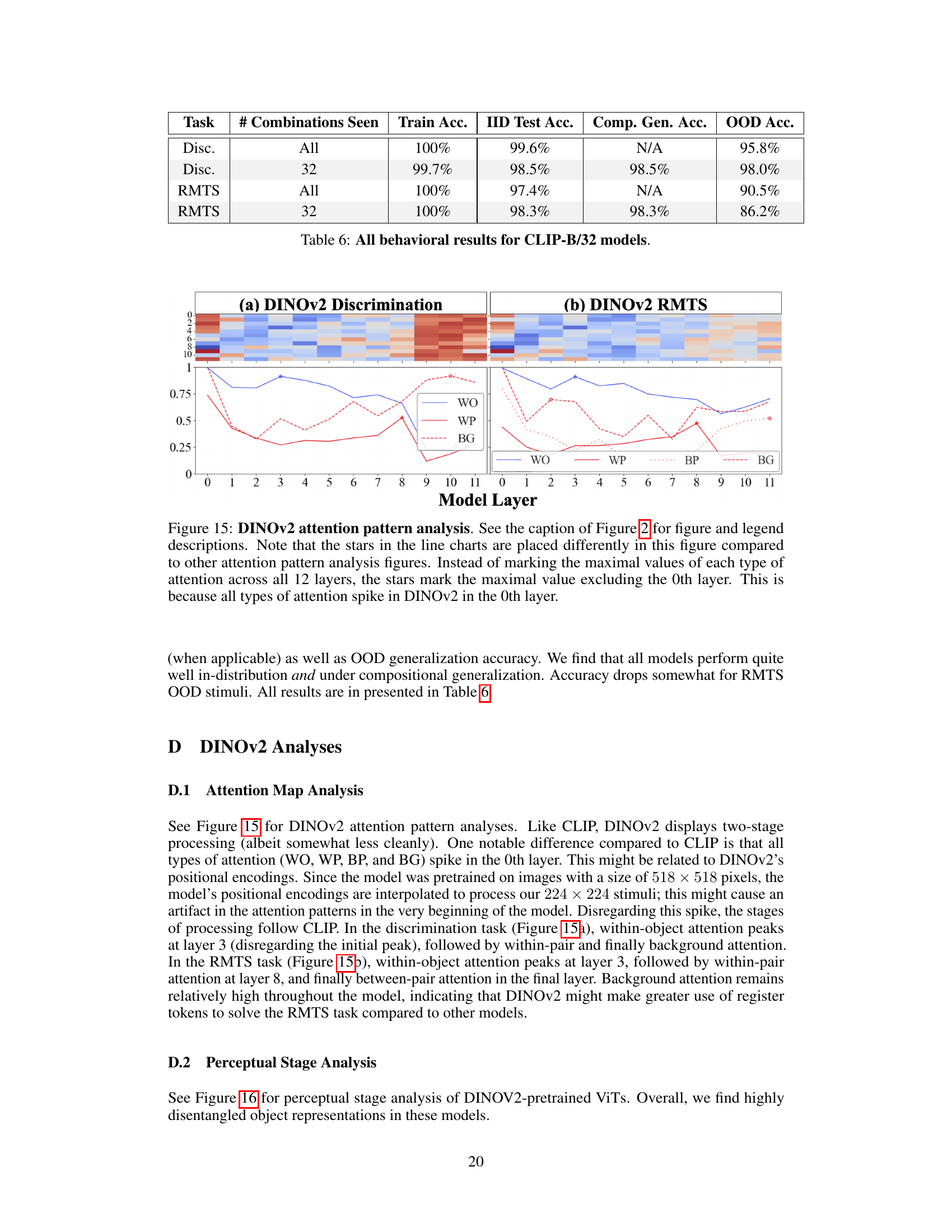
🔼 This table presents the performance of CLIP-B/32 models on discrimination and RMTS tasks. The performance is measured across different training conditions: using all 256 shape-color combinations or a subset of 32, and evaluated on in-distribution (IID), compositional generalization, and out-of-distribution (OOD) test sets. The metrics presented are training accuracy, IID test accuracy, compositional generalization accuracy, and OOD accuracy.
read the caption
Table 6: All behavioral results for CLIP-B/32 models.

🔼 This table presents the performance of Vision Transformers (ViTs) trained from scratch on the discrimination task using auxiliary losses. It shows how adding disentanglement and pipeline losses impacts training accuracy, test accuracy (on IID data), and compositional generalization accuracy. The results demonstrate that adding auxiliary losses significantly improves performance, highlighting the importance of both disentangled representations and a two-stage processing pipeline in solving this visual relational reasoning task.
read the caption
Table 7: Performance of ViTs trained from scratch on the discrimination task with auxiliary losses.
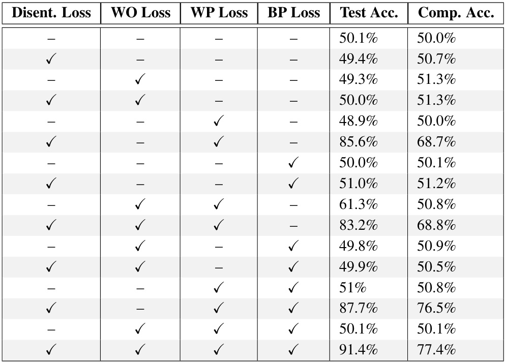
🔼 This table presents the results of experiments using Vision Transformers (ViTs) trained from scratch on same-different tasks. The impact of adding auxiliary loss functions (disentanglement loss and pipeline loss) on the model’s performance is evaluated for both discrimination and relational match-to-sample (RMTS) tasks. It shows that adding these losses improves accuracy, particularly when both are used together for the RMTS task, demonstrating the benefit of encouraging disentanglement and two-stage processing.
read the caption
Table 1: Performance of ViTs trained from scratch with auxiliary losses. Adding either a disentanglement loss term to encourage disentangled object representations (Disent. Loss) or a pipeline loss to encourage two-stage processing in the attention heads (Pipeline Loss) boosts test accuracy and compositional generalization (Comp. Acc.) for the discrimination task. Both auxiliary losses are required to boost accuracy for the RMTS task.
Full paper#
