An Autoencoder-Like Nonnegative Matrix Co-Factorization for Improved Student Cognitive Modeling

8UqyWNsnyA

Shenbao Yu et el.

TL;DR
#

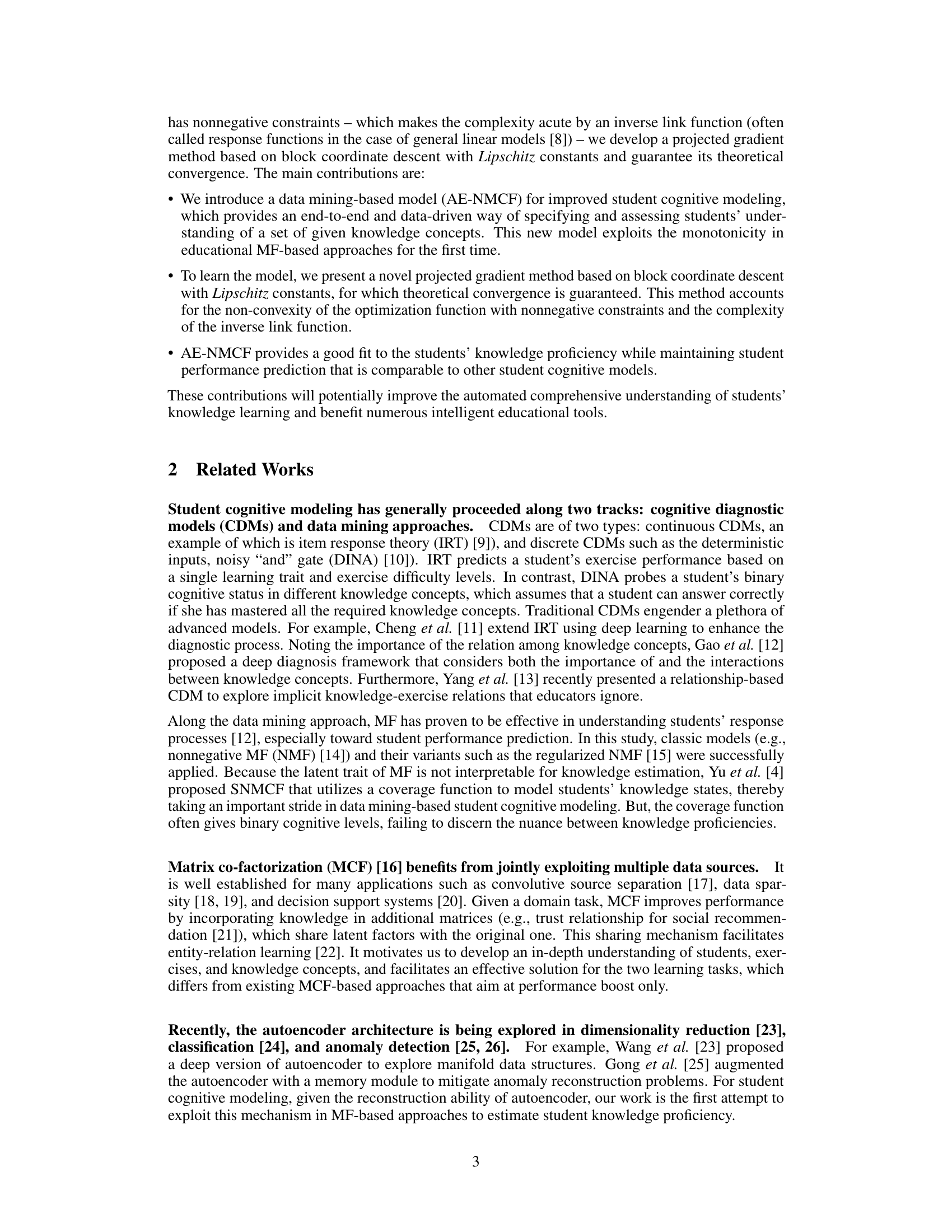
Student cognitive modeling (SCM) aims to predict student performance and knowledge proficiency, but existing methods struggle with sparse data and inaccurate proficiency estimation. Traditional matrix factorization techniques can predict performance well but fail to estimate knowledge levels reliably, often resulting in cascading errors in prediction. Cognitive diagnosis models (CDMs) provide detailed insights but rely on handcrafted features that might not capture the nuances of actual cognitive functioning.

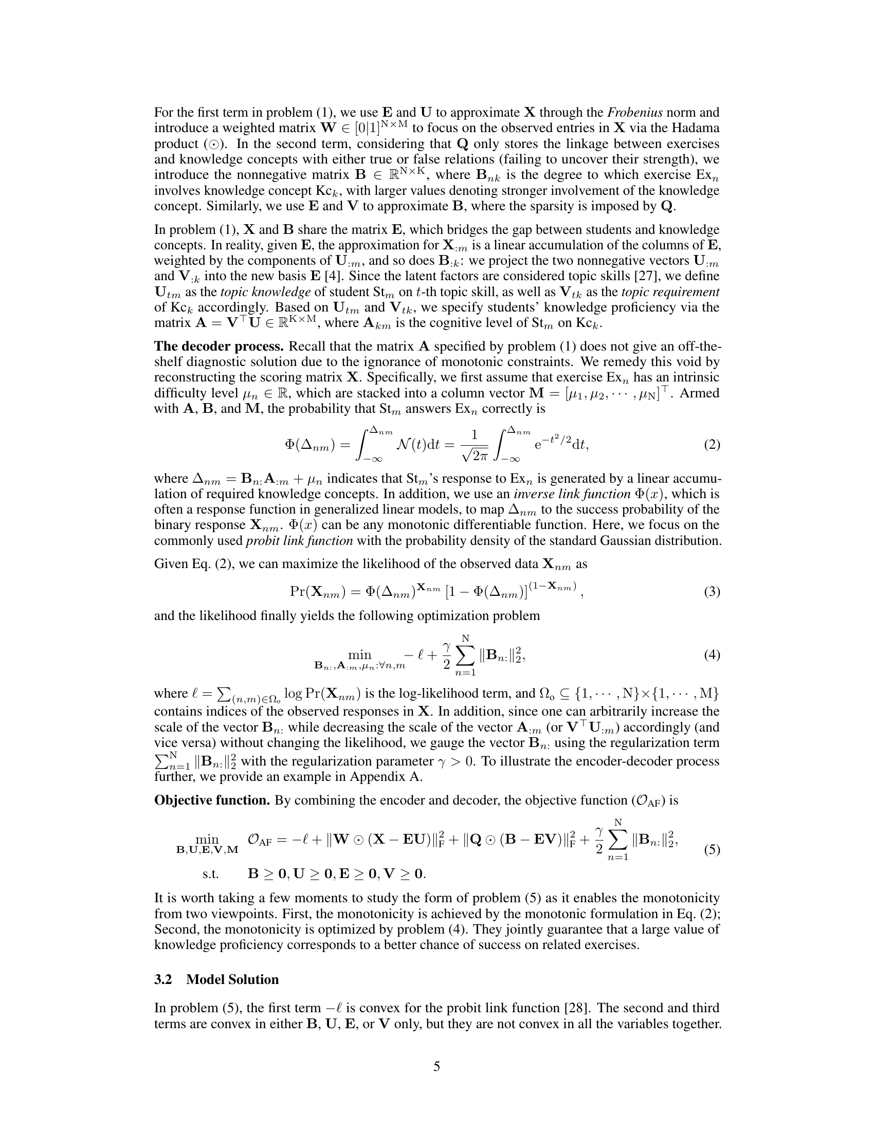
This paper introduces AE-NMCF, an autoencoder-like nonnegative matrix co-factorization method. AE-NMCF integrates monotonicity, a fundamental psychometric theory, into a co-factorization framework using an encoder-decoder learning pipeline. This improves the accuracy of knowledge proficiency estimation. A projected gradient method is developed with guaranteed convergence, and experiments show improved accuracy and ability in estimating knowledge over existing models, improving both prediction and diagnosis simultaneously.

Key Takeaways
#

Why does it matter?
#

This paper is important because it presents a novel approach to student cognitive modeling, improving the accuracy of estimating knowledge proficiency. This is crucial for personalized learning and educational resource allocation. The autoencoder-like framework and projected gradient method offer a new way to analyze student learning data, opening new avenues for research. Its interpretable results are also highly valuable for educators and researchers.

Visual Insights
#

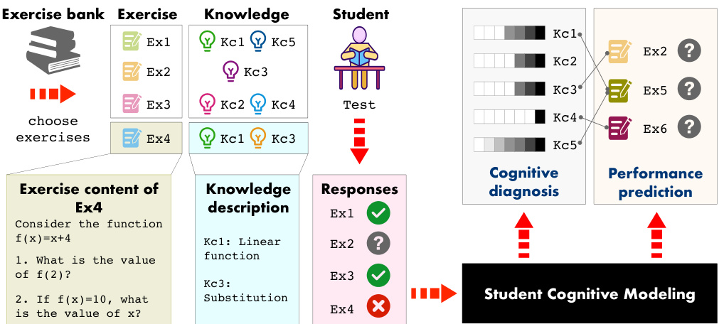
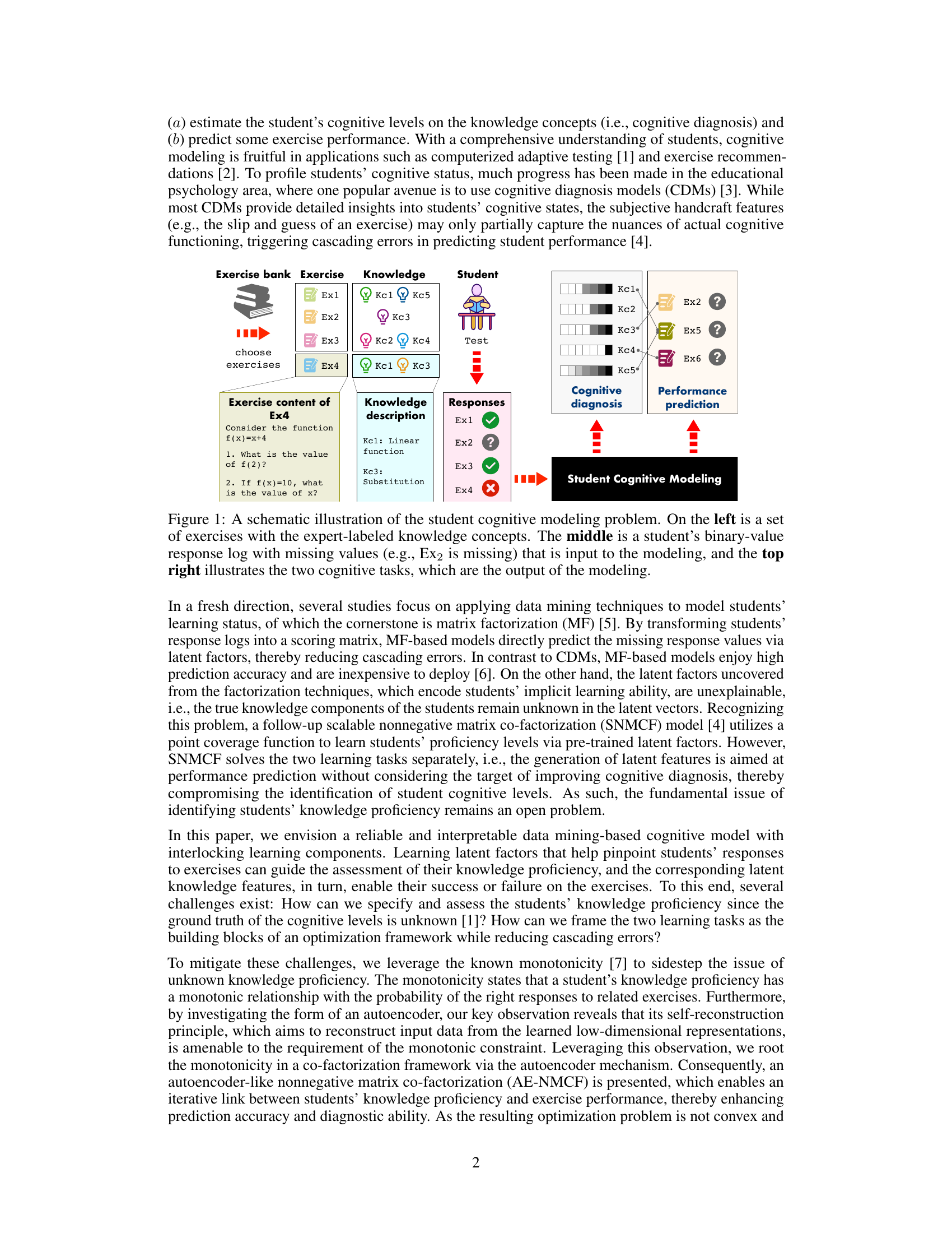
🔼 This figure illustrates the student cognitive modeling problem. It shows an exercise bank with exercises and their associated knowledge concepts. A student interacts with the exercises, providing binary responses (correct/incorrect). The model then performs two tasks using the response log: it predicts student performance on exercises they haven’t attempted (Performance Prediction) and diagnoses the student’s knowledge proficiency in each knowledge concept (Cognitive Diagnosis). The missing values in the student’s response log represent exercises the student hasn’t yet attempted.
read the caption
Figure 1: A schematic illustration of the student cognitive modeling problem. On the left is a set of exercises with the expert-labeled knowledge concepts. The middle is a student's binary-value response log with missing values (e.g., Ex2 is missing) that is input to the modeling, and the top right illustrates the two cognitive tasks, which are the output of the modeling.

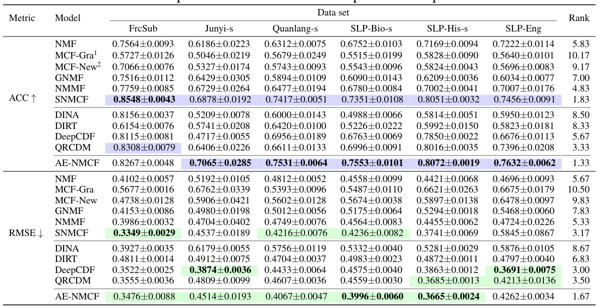
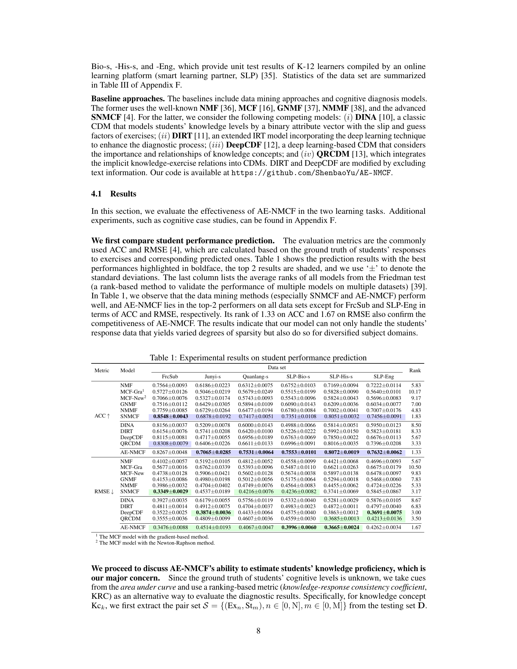
🔼 This table presents the results of student performance prediction using various models, including AE-NMCF and several baselines. The metrics used are Accuracy (ACC) and Root Mean Squared Error (RMSE). The table shows the performance of each model across six different datasets, highlighting the top two performers in boldface. The average ranks of the models from a Friedman test (a statistical test for comparing multiple models) are also included.
read the caption
Table 1: Experimental results on student performance prediction

In-depth insights
#

AE-NMCF Model
#

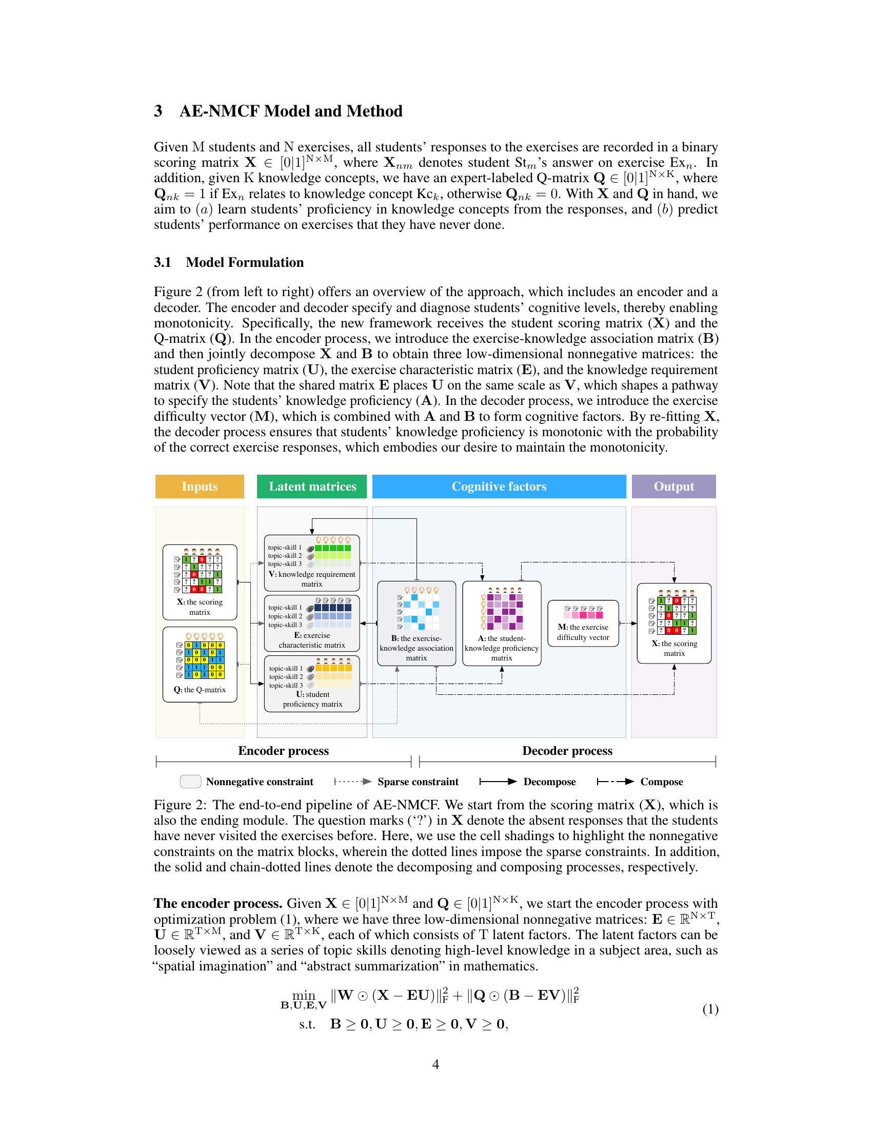
The AE-NMCF model, an autoencoder-like nonnegative matrix co-factorization, presents a novel approach to student cognitive modeling. It leverages the monotonicity principle, a fundamental psychometric theory, to improve the accuracy of estimating students’ knowledge proficiency. Unlike traditional methods that treat performance prediction and cognitive diagnosis as separate tasks, AE-NMCF integrates these tasks in an encoder-decoder framework. The encoder decomposes the student response matrix and the exercise-knowledge matrix to learn latent representations of student proficiency and exercise characteristics. The decoder then reconstructs the response matrix, enforcing monotonicity. The model’s architecture effectively addresses the sparsity challenge, commonly encountered in educational data, and offers an end-to-end data-driven approach. A key strength is the incorporation of nonnegative constraints and the use of a projected gradient method for optimization, ensuring theoretical convergence. The results show its effectiveness across different datasets and subjects, improving both predictive accuracy and diagnostic ability. The model’s interpretability, owing to its reliance on monotonicity and a clear framework, allows for insightful analysis of student learning.

Monotonicity in SCM
#

In student cognitive modeling (SCM), monotonicity is a crucial psychometric property signifying that a student’s proficiency in a specific knowledge concept should monotonically increase the probability of successfully answering related exercises. This principle is inherently intuitive and reasonable, implying better proficiency leads to higher accuracy. Many SCM approaches, like matrix factorization, implicitly assume or aim for this characteristic, but often lack explicit mechanisms to enforce or leverage monotonicity effectively. The paper’s innovation centers around this concept, specifically by embedding monotonicity directly into the model architecture. This approach not only leads to more accurate and reliable student proficiency estimates but also improves exercise performance prediction. By directly incorporating monotonicity, the model avoids cascading errors and better captures nuanced relationships between student knowledge and exercise responses. The success is further highlighted by the superiority of AE-NMCF in capturing this relationship, as demonstrated through the experimental results. This emphasis on monotonicity represents a significant advancement in SCM, moving beyond simple correlation to a more principled, interpretable modeling framework.

PG-BCD+Lipschitz
#

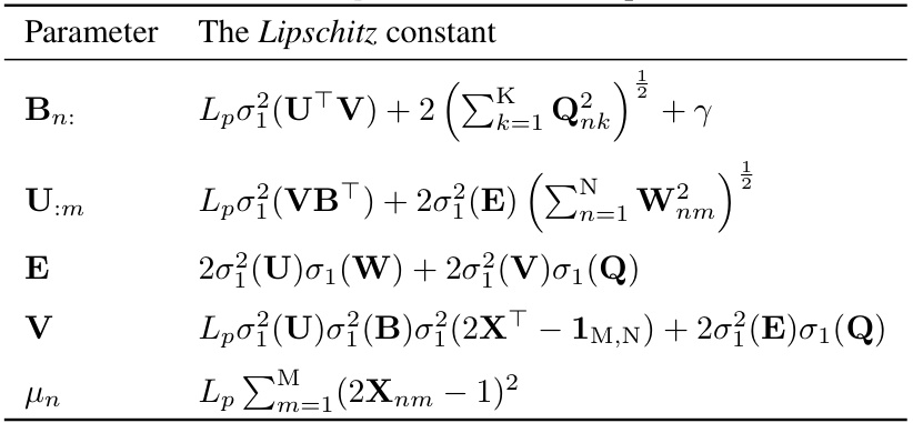
The heading ‘PG-BCD+Lipschitz’ suggests an optimization algorithm combining projected gradient descent (PG), a method for handling constrained optimization problems, with block coordinate descent (BCD), an iterative approach that updates one block of variables at a time. The addition of ‘+Lipschitz’ indicates that the algorithm incorporates Lipschitz continuity in its convergence analysis or step size selection. This is crucial for non-convex optimization problems because it provides a way to guarantee convergence even when the objective function’s gradient is not uniformly smooth. Lipschitz continuity ensures bounded changes in the gradient, enabling controlled step sizes and preventing divergence. Therefore, PG-BCD+Lipschitz likely offers an efficient way to solve challenging, non-convex optimization problems with non-negativity constraints, as frequently encountered in machine learning applications like non-negative matrix factorization. The algorithm’s design highlights a focus on theoretical guarantees and practical efficiency.

Knowledge Estimation
#

The core of this research lies in improving student knowledge estimation, a critical task within student cognitive modeling (SCM). The paper challenges the limitations of existing SCM approaches, particularly in scenarios with sparse student-exercise interaction data. It proposes a novel autoencoder-like nonnegative matrix co-factorization (AE-NMCF) method to address these limitations. AE-NMCF leverages an encoder-decoder structure and incorporates the psychometric theory of monotonicity to indirectly estimate knowledge proficiency. This clever approach avoids the need for ground truth knowledge labels, thus making it more robust and widely applicable. By jointly optimizing prediction accuracy and knowledge estimation, AE-NMCF offers a significant improvement over existing methods. The monotonicity constraint, embedded within the model, ensures that better knowledge proficiency is consistently associated with higher performance on related exercises, adding a layer of interpretability. Finally, the development of a projected gradient method guarantees the theoretical convergence of the proposed algorithm, enhancing its reliability and practical applicability.

Future Works
#

The paper’s conclusion mentions future work directions, focusing on enhancing the model’s capabilities and addressing limitations. Exploring the learning dependencies between knowledge concepts is crucial, as the current model doesn’t explicitly capture prerequisite relationships. This improvement could significantly enhance the accuracy and interpretability of knowledge proficiency estimations. Secondly, investigating alternative and more efficient parameter learning methods is important. The current approach, while effective, may present scalability challenges with larger datasets. The exploration of alternative methods, possibly incorporating recent advancements in optimization, could lead to faster training and improved convergence properties. Finally, evaluating the model’s robustness and performance under diverse conditions is essential. More extensive testing, including its applicability across different subject domains and varying data sparsity levels, will further solidify the model’s validity and generalizability.

More visual insights
#

More on figures

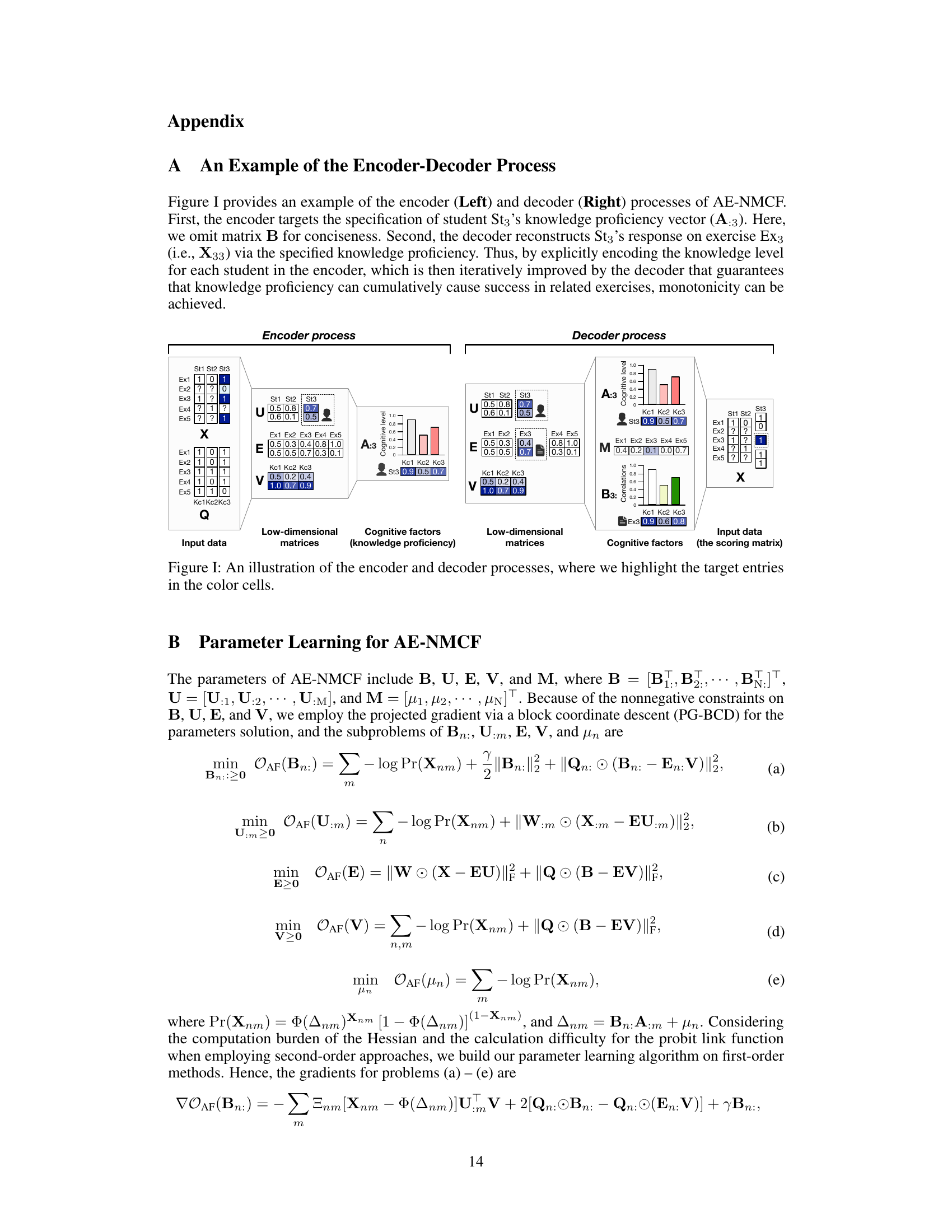
🔼 This figure illustrates the AE-NMCF model’s architecture. It shows the inputs (scoring matrix X and Q-matrix Q), the encoder process (decomposing X and B into U, E, and V matrices), the decoder process (combining A, B, and M to reconstruct X), and the outputs (reconstructed scoring matrix X). The figure highlights the nonnegative and sparse constraints in the model. The encoder learns latent features representing student proficiency and exercise characteristics. The decoder uses these features to predict student performance. The overall process is designed to be end-to-end and address the issue of missing data and monotonicity in student response.
read the caption
Figure 2: The end-to-end pipeline of AE-NMCF. We start from the scoring matrix (X), which is also the ending module. The question marks ('?') in X denote the absent responses that the students have never visited the exercises before. Here, we use the cell shadings to highlight the nonnegative constraints on the matrix blocks, wherein the dotted lines impose the sparse constraints. In addition, the solid and chain-dotted lines denote the decomposing and composing processes, respectively.

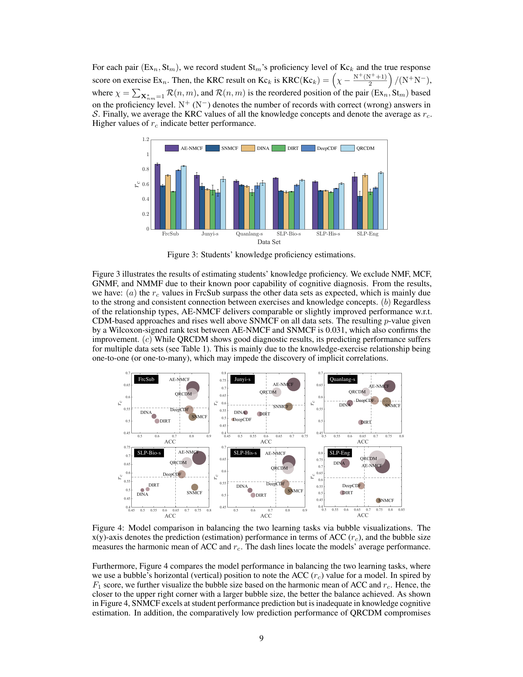
🔼 This figure compares the performance of different models in estimating students’ knowledge proficiency using the KRC metric. Higher KRC values indicate better performance. The models compared include AE-NMCF, SNMCF, DINA, DIRT, DeepCDF, and QRCDM. The figure shows the average KRC scores across multiple datasets for each model, allowing for a comparison of their relative diagnostic abilities.
read the caption
Figure 3: Students' knowledge proficiency estimations.

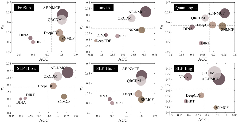
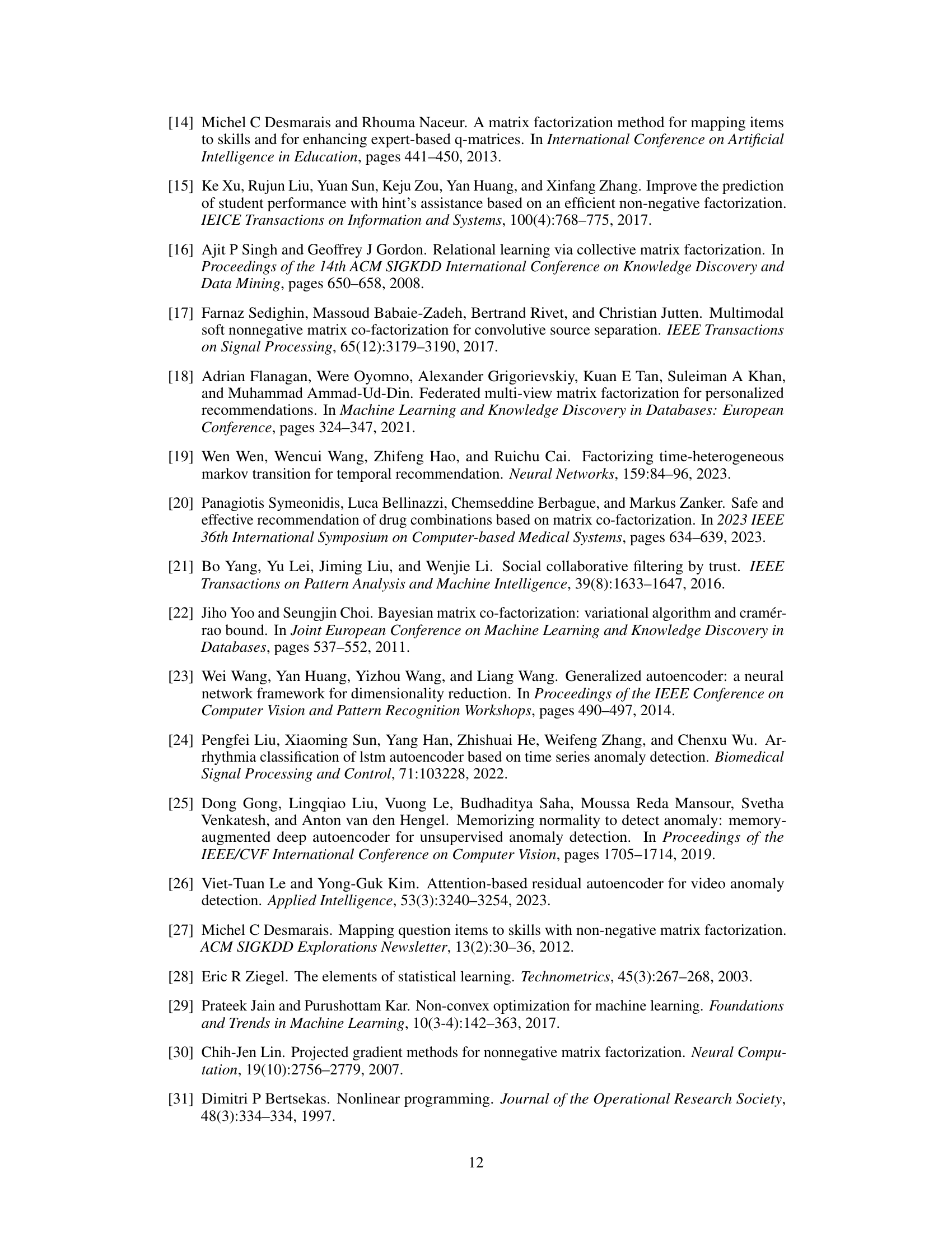
🔼 This figure visualizes the performance of different models in balancing prediction accuracy (ACC) and knowledge proficiency estimation ability (rc). Each model is represented by a bubble, with the x-coordinate representing ACC, the y-coordinate representing rc, and the bubble size reflecting the harmonic mean of ACC and rc. Larger bubbles indicate better balance between prediction accuracy and estimation ability. The figure helps compare the overall performance of different models across these two key aspects of student cognitive modeling.
read the caption
Figure 4: Model comparison in balancing the two learning tasks via bubble visualizations. The x(y)-axis denotes the prediction (estimation) performance in terms of ACC (rc), and the bubble size measures the harmonic mean of ACC and rc. The dash lines locate the models' average performance.

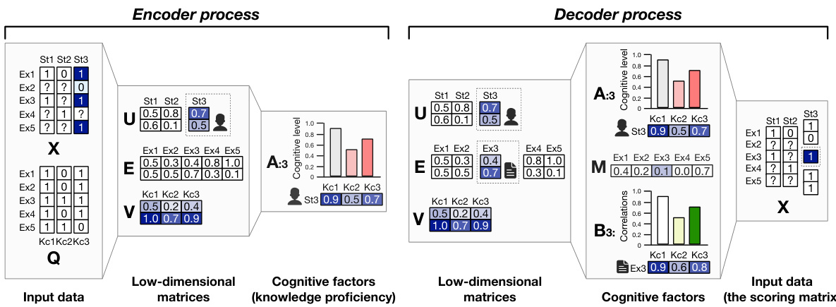
🔼 This figure illustrates the end-to-end pipeline of the proposed AE-NMCF model for student cognitive modeling. It shows how the model processes the input data (student responses and exercise-knowledge associations) through an encoder and decoder to estimate student knowledge proficiency and predict their performance on unseen exercises. The encoder decomposes the input matrices into lower-dimensional latent matrices, which capture the underlying relationships between students, exercises, and knowledge concepts. The decoder then reconstructs the original scoring matrix, enforcing monotonicity to ensure that a student’s proficiency level is reflected in their performance. Non-negative constraints are also highlighted, demonstrating how the model handles the sparsity in student responses.
read the caption
Figure 2: The end-to-end pipeline of AE-NMCF. We start from the scoring matrix (X), which is also the ending module. The question marks ('?') in X denote the absent responses that the students have never visited the exercises before. Here, we use the cell shadings to highlight the nonnegative constraints on the matrix blocks, wherein the dotted lines impose the sparse constraints. In addition, the solid and chain-dotted lines denote the decomposing and composing processes, respectively.

🔼 This figure illustrates the AE-NMCF model’s pipeline, which consists of an encoder and a decoder. The encoder takes the student’s response matrix (X) and Q-matrix (Q), which describes the relationship between exercises and knowledge concepts, as input and decomposes them into latent matrices (U, E, V). These latent matrices capture students’ proficiency in knowledge concepts and the characteristics of exercises. The encoder then combines these factors to produce a student-knowledge proficiency matrix (A). The decoder takes A, exercise difficulty vector (M), and the Q-matrix as input. It then reconstructs the original response matrix (X). The process includes nonnegative and sparse constraints, ensuring monotonicity and handling missing values in the original data.
read the caption
Figure 2: The end-to-end pipeline of AE-NMCF. We start from the scoring matrix (X), which is also the ending module. The question marks ('?') in X denote the absent responses that the students have never visited the exercises before. Here, we use the cell shadings to highlight the nonnegative constraints on the matrix blocks, wherein the dotted lines impose the sparse constraints. In addition, the solid and chain-dotted lines denote the decomposing and composing processes, respectively.

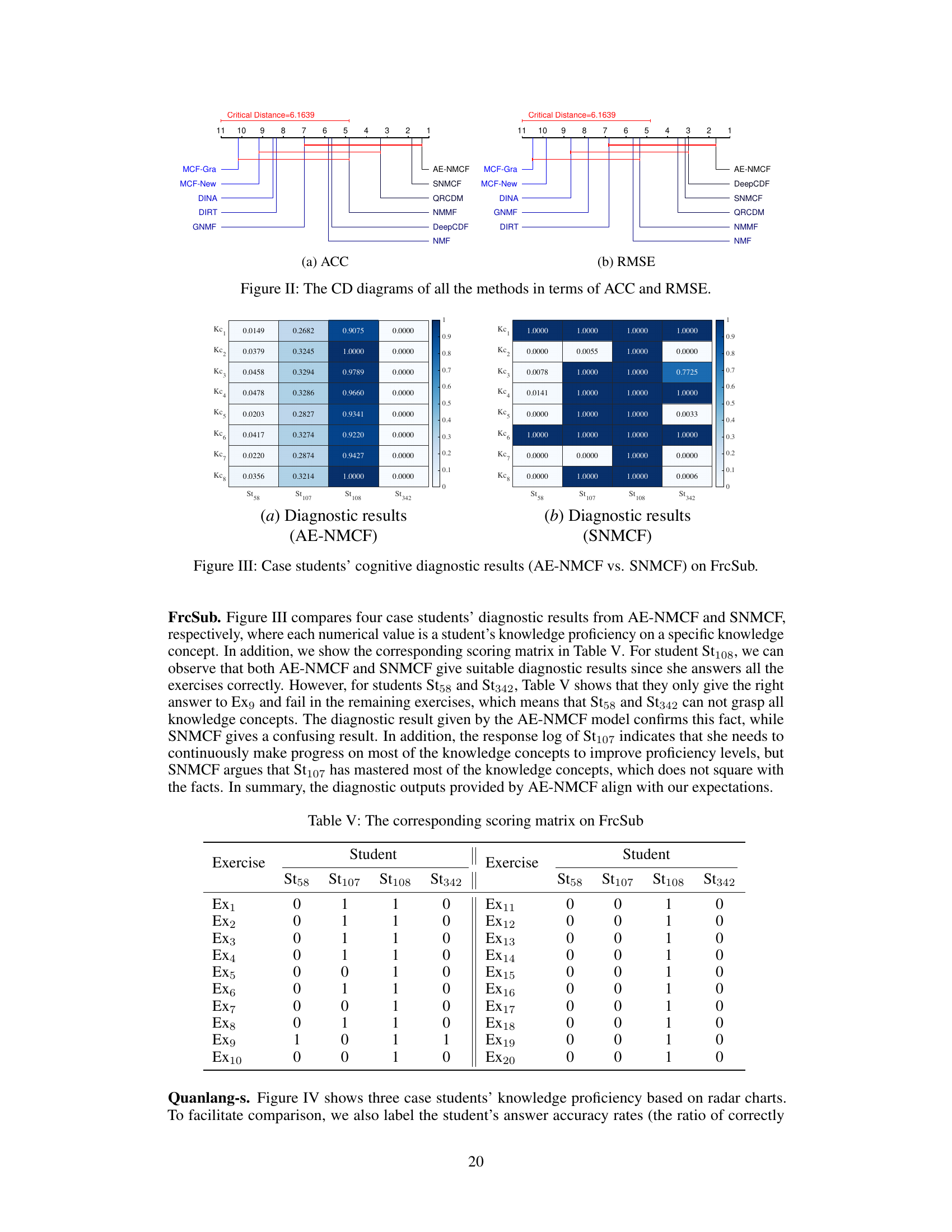
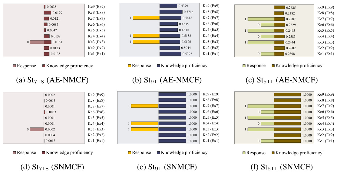
🔼 This figure compares the cognitive diagnostic results of four students obtained from AE-NMCF and SNMCF models on the FrcSub dataset. Each heatmap shows the estimated knowledge proficiency of each student for each of the knowledge concepts. The color intensity represents the proficiency level, with darker colors indicating higher proficiency. The corresponding scoring matrix is provided in Table V. The comparison highlights the differences in diagnostic accuracy between the two models, particularly for students with inconsistent performance across exercises, illustrating the ability of AE-NMCF to provide more reliable and interpretable results.
read the caption
Figure III: Case students’ cognitive diagnostic results (AE-NMCF vs. SNMCF) on FrcSub.

🔼 This figure shows a comparison of the diagnostic results for three students (St50, St33, and St42) obtained using both AE-NMCF and SNMCF models on the Quanlang-s dataset. Each radar chart represents a student, with each axis representing a knowledge concept (Kc). The distance from the center to the edge of each radar chart corresponds to the student’s knowledge proficiency level for that specific concept. The different colors represent different models: AE-NMCF and SNMCF. This visualization helps to compare the diagnostic capabilities of the two models for individual students and across different knowledge concepts, highlighting areas where one model might perform better than the other.
read the caption
Figure IV: Diagnosis results of three case students between AE-NMCF and SNMCF on Quanlang-s.

🔼 This figure illustrates the end-to-end pipeline of the AE-NMCF model. It shows how the model takes student response data (X), exercise-knowledge associations (Q), and pre-trained latent matrices as input. The encoder processes this data to generate low-dimensional matrices representing student proficiency (U), exercise characteristics (E), and knowledge requirements (V), resulting in a student-knowledge proficiency matrix (A). This matrix, along with exercise difficulty (M), is fed into the decoder to reconstruct the original scoring matrix (X), ensuring the monotonicity constraint. The figure highlights nonnegative constraints and the sparse nature of the data through visual cues.
read the caption
Figure 2: The end-to-end pipeline of AE-NMCF. We start from the scoring matrix (X), which is also the ending module. The question marks ('?') in X denote the absent responses that the students have never visited the exercises before. Here, we use the cell shadings to highlight the nonnegative constraints on the matrix blocks, wherein the dotted lines impose the sparse constraints. In addition, the solid and chain-dotted lines denote the decomposing and composing processes, respectively.

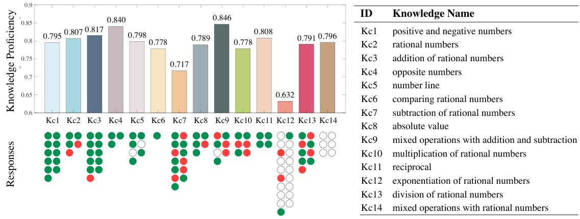
🔼 This figure visualizes the diagnostic results for a single student on the Quanlang-s dataset using the AE-NMCF model. The top bar chart displays the student’s estimated knowledge proficiency levels for each of the 14 knowledge concepts. Below, a dot plot shows the student’s responses to exercises related to each concept; green dots represent correct answers, red dots represent incorrect answers, and hollow circles indicate unanswered exercises. The figure provides an easily interpretable view of a student’s knowledge strengths and weaknesses, highlighting areas where the student performed well and areas needing improvement.
read the caption
Figure 6: Diagnosis visualization of a case student on Quanlang-s via AE-NMCF. The bottom left shows her responses to related exercises. The circles with green (red) colors represent right (wrong) responses, and the hollow circles denote the absent responses.

🔼 This figure illustrates the AE-NMCF model’s architecture, which consists of an encoder and a decoder. The encoder takes the student-exercise response matrix (X) and the Q-matrix (exercise-knowledge concept relationship) as input. It decomposes these into lower-dimensional matrices representing student proficiency (U), exercise characteristics (E), and knowledge concept requirements (V). These latent factors are then used by the decoder to reconstruct the original response matrix (X), incorporating exercise difficulty (M) and enforcing monotonicity through a linear accumulation of required knowledge concepts. Missing entries in X are predicted by the decoder.
read the caption
Figure 2: The end-to-end pipeline of AE-NMCF. We start from the scoring matrix (X), which is also the ending module. The question marks ('?') in X denote the absent responses that the students have never visited the exercises before. Here, we use the cell shadings to highlight the nonnegative constraints on the matrix blocks, wherein the dotted lines impose the sparse constraints. In addition, the solid and chain-dotted lines denote the decomposing and composing processes, respectively.

🔼 This figure illustrates the AE-NMCF model’s architecture, highlighting its encoder and decoder components. The encoder processes the student’s response matrix and the exercise-knowledge association matrix to generate latent matrices representing student proficiency, exercise characteristics, and knowledge requirements. The decoder then uses these latent matrices and an exercise difficulty vector to reconstruct the original response matrix, ensuring monotonicity between student knowledge proficiency and performance.
read the caption
Figure 2: The end-to-end pipeline of AE-NMCF. We start from the scoring matrix (X), which is also the ending module. The question marks ('?') in X denote the absent responses that the students have never visited the exercises before. Here, we use the cell shadings to highlight the nonnegative constraints on the matrix blocks, wherein the dotted lines impose the sparse constraints. In addition, the solid and chain-dotted lines denote the decomposing and composing processes, respectively.

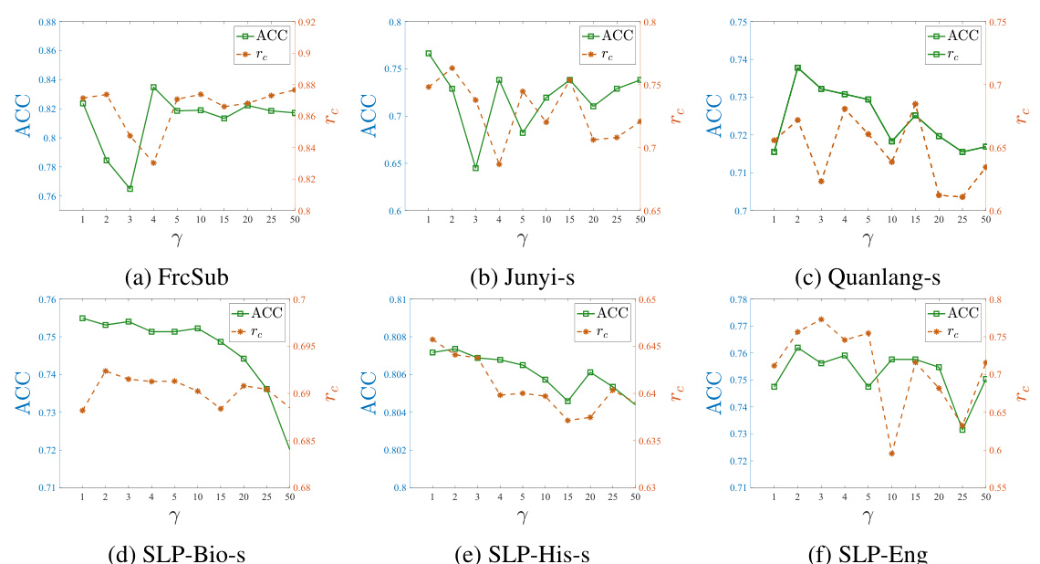
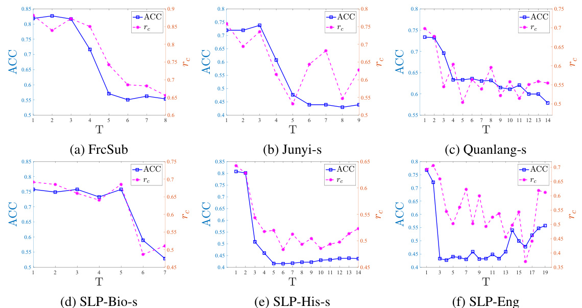
🔼 The figure shows the sensitivity analysis of parameter T (number of latent factors) on different datasets. For each dataset, the ACC (accuracy) and rc (knowledge-response consistency coefficient) are plotted against different values of T. The results suggest that there is an optimal value of T for each dataset, where increasing T beyond this optimal value leads to a decrease in both ACC and rc.
read the caption
Figure VIII: Sensitivity analysis of parameter T on the data sets.