TL;DR#
This research explores the theoretical feasibility of learning high-dimensional data using models with far fewer parameters than dimensions. The paper investigates whether gradient flow (a continuous version of gradient descent) can successfully train such underparameterized models. A key challenge is that, with a small number of parameters, the model’s loss function tends to have many undesirable local minima, hindering the training process. This issue was tackled using a variety of mathematical approaches and techniques.
The study reveals a surprising result: Two-parameter models can achieve high success probability in learning high-dimensional targets. However, this is achievable only under specific conditions. The paper shows that underparameterized models are fundamentally limited, meaning there exist large sets of non-learnable targets in high-dimensional spaces. Specifically, the set of learnable targets is not dense in the target space, and any subset homeomorphic to the parameter space’s sphere contains non-learnable targets. Importantly, the model demonstrating effective two-parameter learning is structurally complex and cannot be expressed by elementary functions.
Key Takeaways#
Why does it matter?#
This paper challenges the common assumption that high-dimensional data requires high-dimensional models. It’s crucial for guiding model design decisions and prompting further research into efficient learning methods. By establishing both positive and negative results, it provides a more complete understanding of the learning dynamics of low-dimensional models with high-dimensional targets, impacting future research on model efficiency and generalization.
Visual Insights#

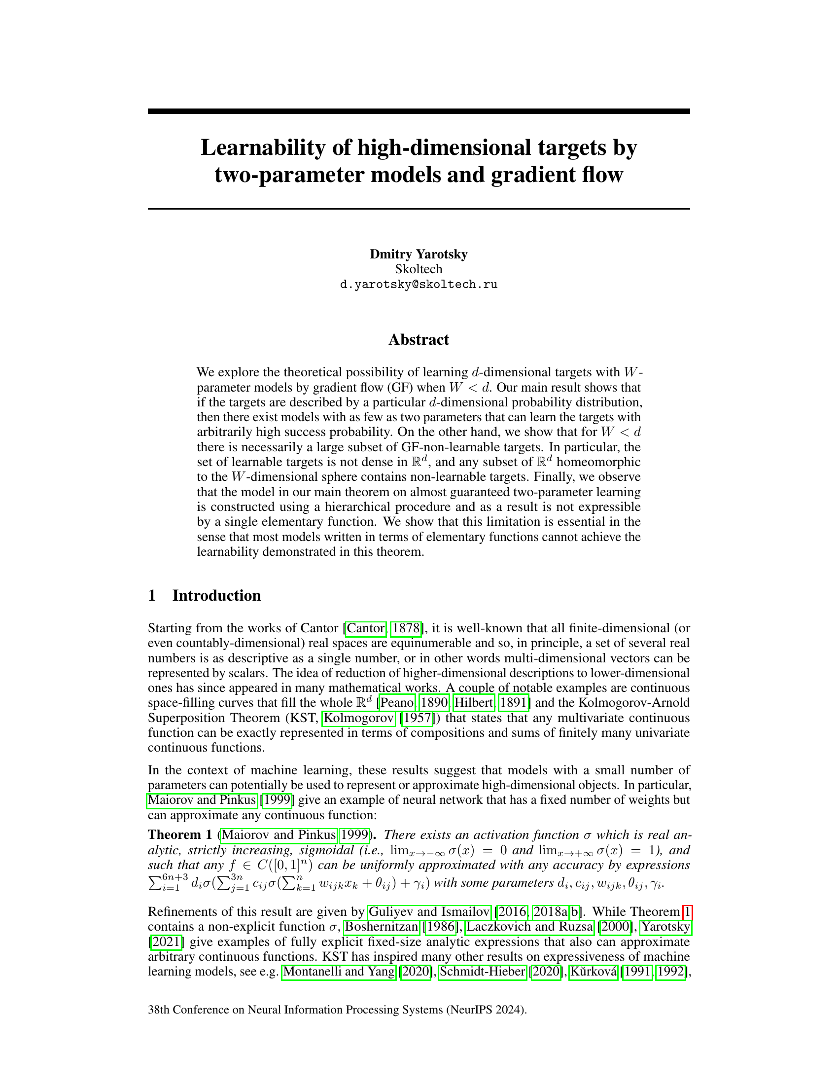
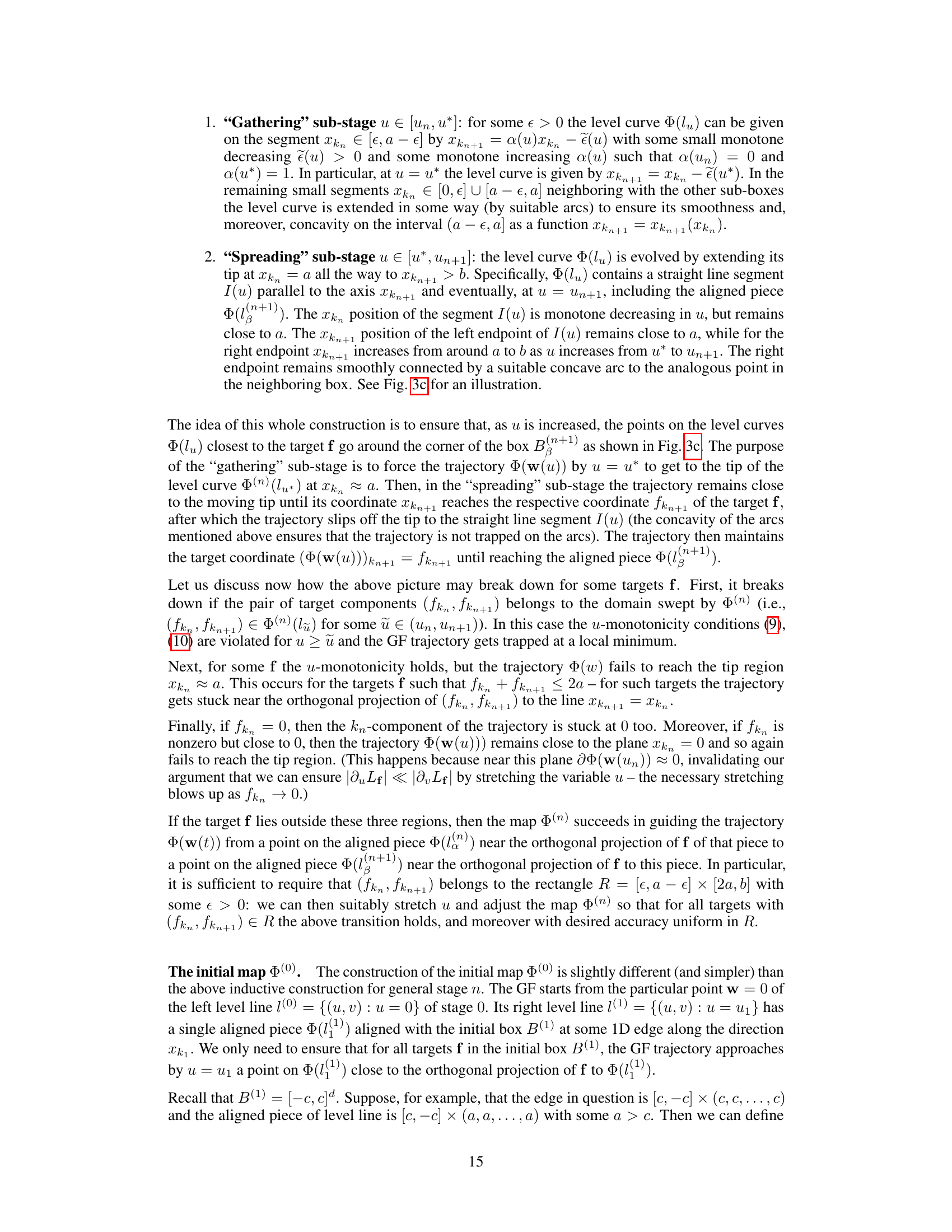
🔼 This figure is a visual aid to understanding Theorem 4, which demonstrates that underparameterization (W<d) in gradient flow (GF) learning severely restricts the set of learnable targets. The figure illustrates that for a set G (homeomorphic to a W-sphere), GF cannot converge for all points in G simultaneously. This is because convergence would require the GF trajectory to be simultaneously close to two antipodal points, g(yt) and g(-yt), which are necessarily far apart.
read the caption
Figure 1: Proof of Theorem 4. GF cannot converge for all points of G: such a convergence would require (zt) to be simultaneously close to both g(yt) and g(-yt), which are far from each other.
In-depth insights#
High-D Target Learning#
High-dimensional target learning explores the challenges and possibilities of training models with fewer parameters than the dimensionality of the target space. A core challenge is the prevalence of spurious local minima, hindering gradient-based optimization methods. The paper investigates whether high-dimensional targets can be learned effectively by models with a limited number of parameters. It shows that while two parameters suffice for learning with high probability under specific conditions, underparameterization fundamentally limits learnability, and the set of learnable targets is not dense. Models expressible as simple functions may not achieve the demonstrated results, suggesting a complex model design is crucial for success in this setting. The research opens avenues for further exploration into model design and the interplay between parameter count, target space, and optimization landscape in high-dimensional learning problems.
Two-Parameter Models#
The study of two-parameter models within the context of high-dimensional target learning presents a fascinating challenge. The core question revolves around the possibility of using such minimally parameterized models to effectively learn complex, high-dimensional data via gradient flow. While intuitively it seems impossible, the paper reveals a surprising result: under specific conditions, and with careful model design, two parameters can suffice for arbitrarily high learning accuracy. This is achieved through a hierarchical model construction that carefully navigates the inherent challenges posed by the low dimensionality and avoids entrapment in suboptimal local minima. However, the limitations of two-parameter models are also demonstrated, highlighting the rarity of situations where they succeed. The authors prove that the set of learnable targets isn’t dense and certain high-dimensional subsets will inherently remain unlearnable, underscoring the delicate balance between the simplicity of a two-parameter model and the complexity of the learning task.
Gradient Flow Limits#
The concept of ‘Gradient Flow Limits’ in the context of machine learning, particularly neural networks, is crucial for understanding the behavior of optimization algorithms. It investigates the asymptotic properties of gradient descent as the number of parameters approaches infinity. Understanding these limits can offer valuable insights into the generalization capabilities and convergence behavior of neural networks. It might reveal whether gradient descent converges to a global minimum or gets trapped in poor local minima, and explain how network architecture and training data influence learning dynamics. Research in this area seeks to bridge the gap between finite-dimensional training and the theoretical understanding of infinite-dimensional settings, thereby providing a more rigorous mathematical framework for analyzing the effectiveness of neural networks and suggesting improvements to optimization strategies. The study of gradient flow limits can uncover fundamental properties of the loss landscape, thereby informing the design of new algorithms and network architectures. Key aspects involve exploring relationships between gradient flow and other theoretical models, such as the Neural Tangent Kernel (NTK) limit, and examining the implications for practical training and generalization performance. This is a vital field of research as it enhances our capacity to effectively train and understand the powerful capabilities of deep neural networks.
Elementary Functions#
The section on elementary functions explores the limitations of using simple functions in approximating high-dimensional targets. It reveals a crucial finding: models relying solely on elementary functions (like polynomials, exponentials, and trigonometric functions) are insufficient for achieving the level of approximation demonstrated in the main theorem. This limitation stems from the inherent constraints of elementary functions, specifically their limited capacity to capture complex, high-dimensional relationships. The authors hypothesize that the hierarchical model, which relies on an infinite procedure, is essential for the success of their approach, making the use of a finite set of elementary functions inadequate. The lack of expressiveness of elementary functions restricts their ability to map low-dimensional parameters to sufficiently complex high-dimensional output spaces, highlighting the need for more sophisticated models capable of handling the inherent complexities of high-dimensional learning.
Future Research#
Future research directions stemming from this work could explore relaxing the strong assumptions made about the target distribution and model structure, investigating the impact on learnability. Further exploration is needed to bridge the gap between theoretical results and practical applications, examining how these findings translate to real-world learning scenarios. This involves studying the effects of noise, finite data sets, and varying degrees of model expressiveness. Investigating the role of optimization algorithms beyond gradient flow would be particularly fruitful. Finally, a crucial area for future research lies in developing novel model architectures specifically designed to overcome the limitations of underparameterized models in learning high-dimensional targets. This could involve exploring hierarchical structures, or fundamentally new approaches inspired by the theoretical findings presented.
More visual insights#
More on figures
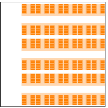
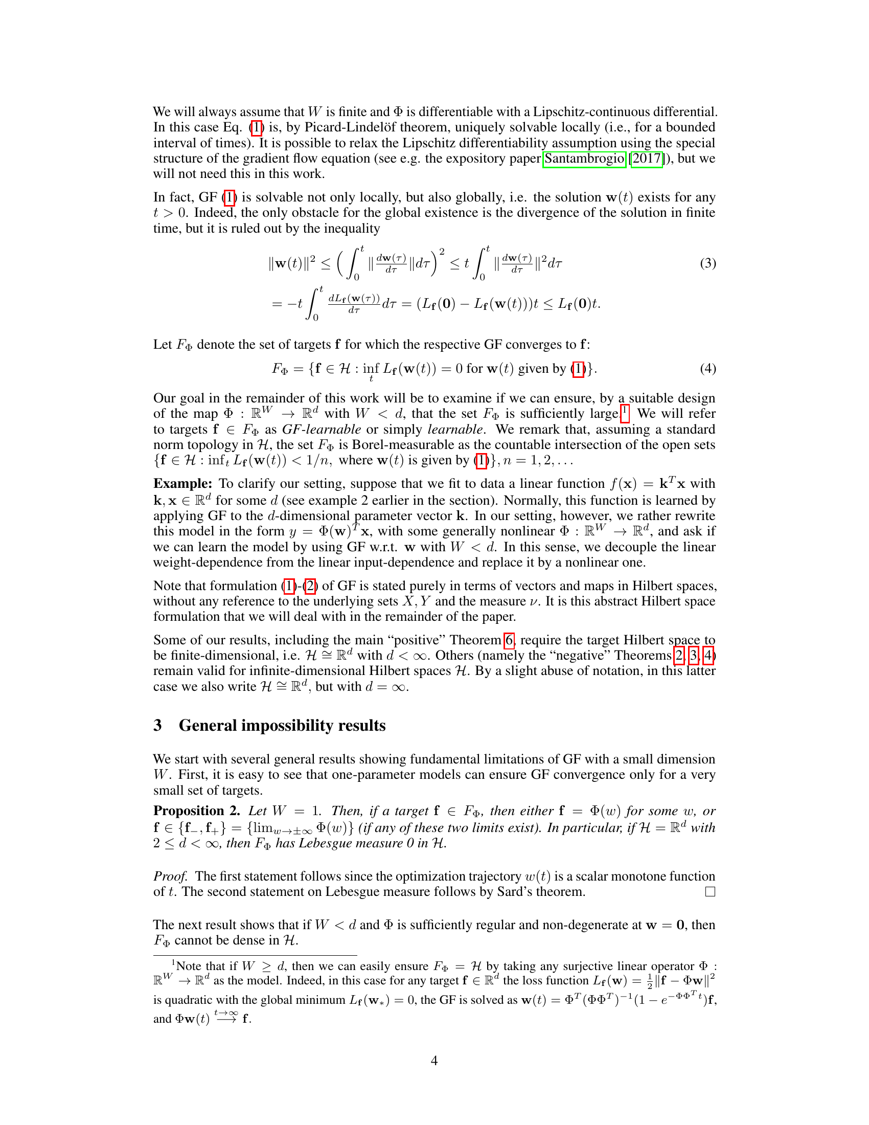
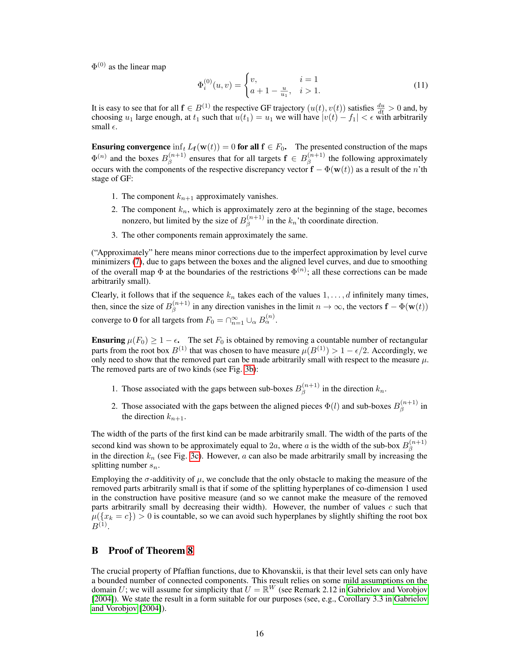
🔼 This figure is a schematic representation of the construction of a multidimensional ‘fat’ Cantor set, denoted as Fo, which is a subset of the learnable targets in Theorem 6 of the paper. This Cantor set is built through a hierarchical process where, at each level n, a set of rectangular boxes B(n) is created. Each box at level n contains several smaller non-intersecting boxes at level n+1. This process is repeated infinitely, resulting in a Cantor set of almost full measure. The boxes are arranged in a grid-like structure, with the indexing ‘a’ representing the individual boxes within a level.
read the caption
Figure 2: In Theorem 6, we ensure that the learnable set of targets F contains a multidimensional 'fat' Cantor set Fo having almost full measure μ. The set Fo has the form Fo = ∩∞n=1 ∪a B(n), where {B(n)}n,a is a nested hierarchy of rectangular boxes in Rd. Here, n is the level of the hierarchy and a is the index of the box within the level.
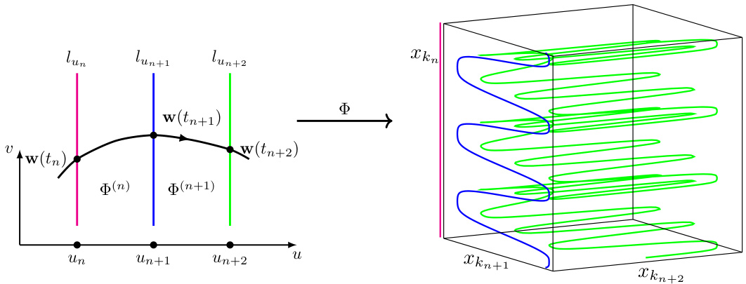
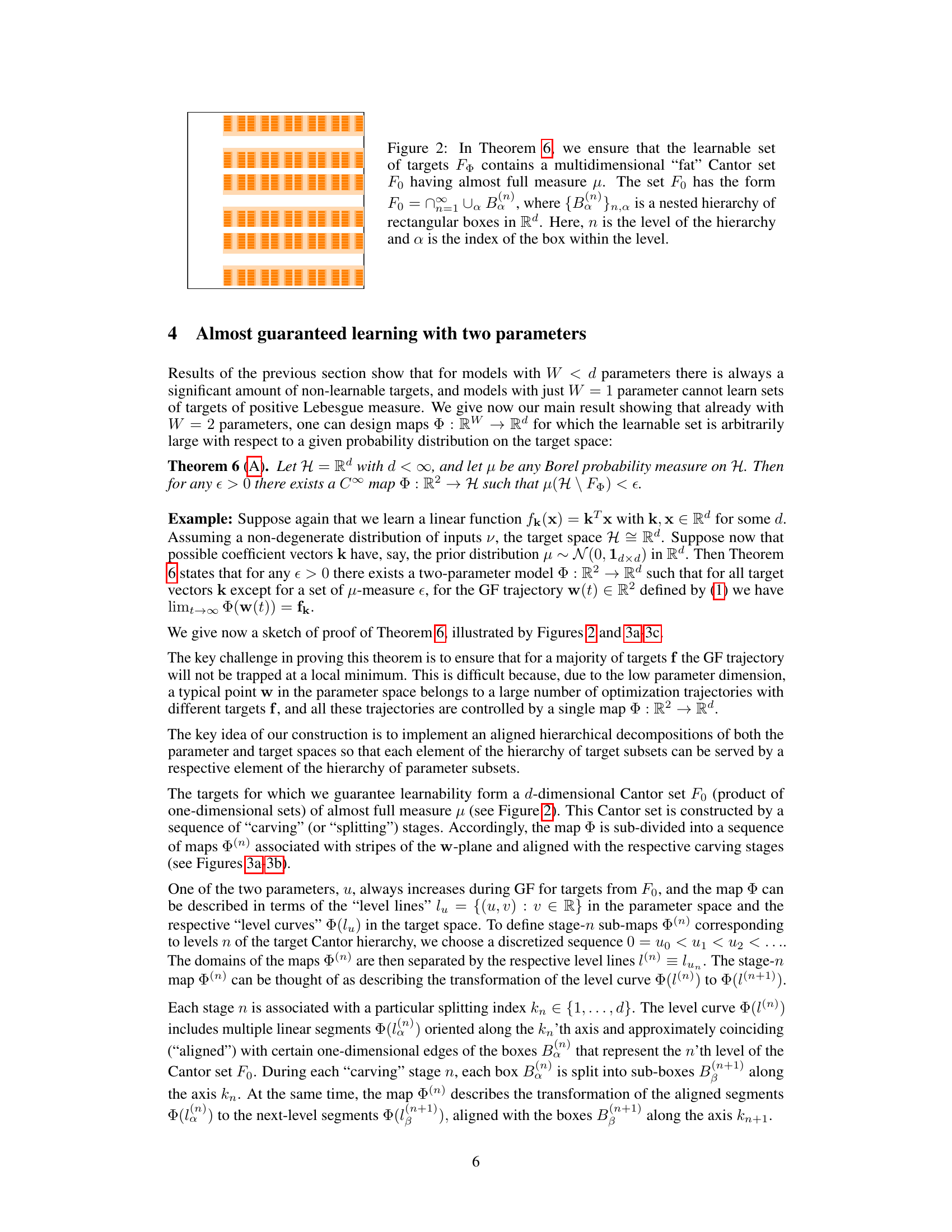
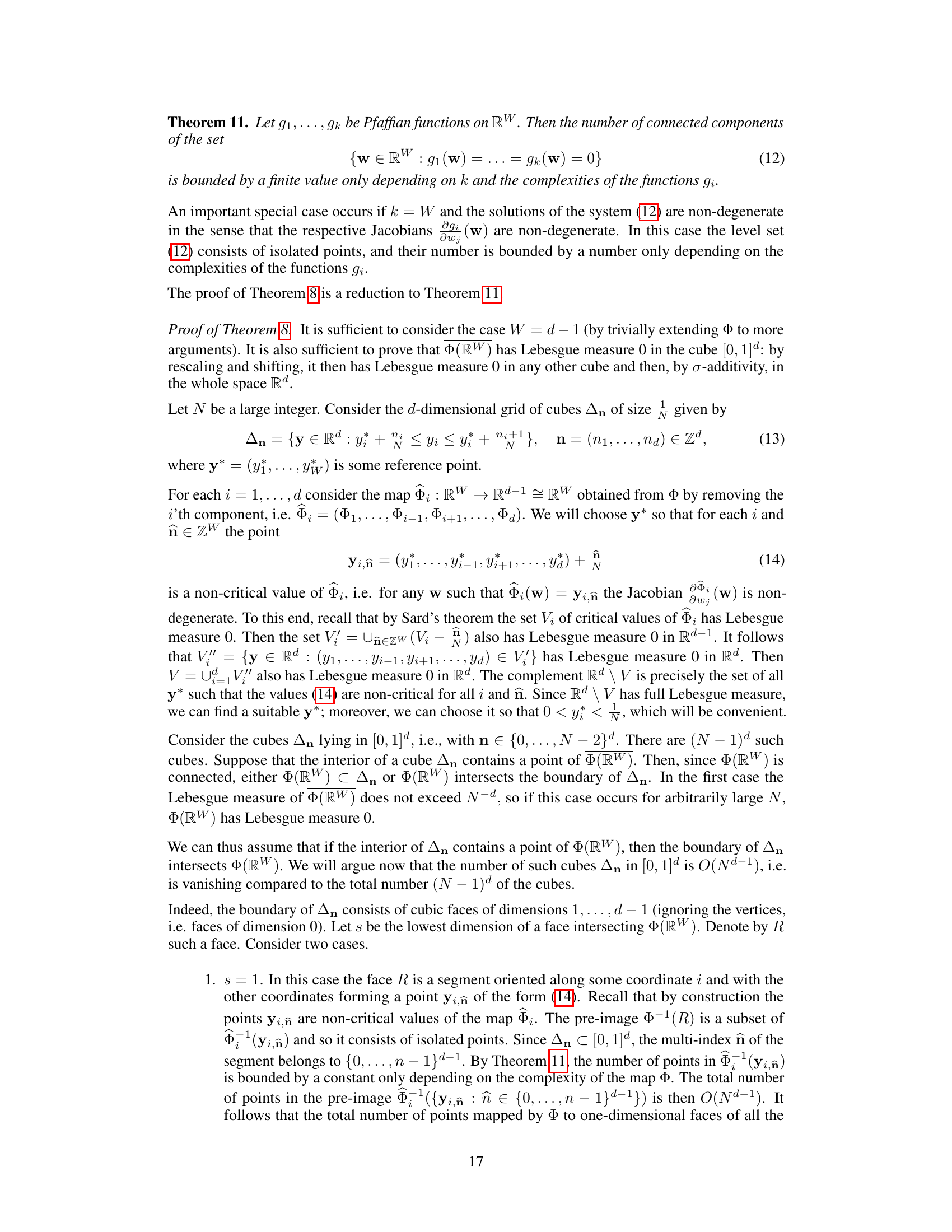
🔼 This figure shows a detailed illustration of the map Φ used in the proof of Theorem 6. It is broken down into three subfigures: (a) Explains the stage-wise decomposition of the map Φ, showing how it’s built from stages Φ(n), level lines l(n), and level curves Φ(l(n)). A GF trajectory passes through these levels. (b) Illustrates box splitting and alignment with curve segments at stage Φ(n). Shows how a parent box B(n) is split into smaller boxes B(n+1), and how aligned segments l(n) are transformed into segments l(n+1). (c) Details the transition from Φ(l(n)) to Φ(l(n+1)) using intermediate curves. It explains how the map ensures that during each stage, a GF trajectory moves towards the target by adjusting coordinates.
read the caption
Figure 3: (a) Stage-wise decomposition of the map Φ. The map Φ is defined by its stages Φ(n) = Φ|un≤u≤un+1 separated by the level lines l(n) = lun = {(u, v) : u = un} and respective level curves Φ(l(n)). Each stage Φ(n) deforms the level curve Φ(l(n)) in the splitting direction xkn+1 to form the new level curve Φ(l(n+1)). A non-exceptional GF trajectory w(t) = (u(t), v(t)) passes through all level lines. The splitting indices kn cycle over the values 1,..., d to ensure convergence w.r.t. each coordinate. (b) Box splitting and curve-box alignment at the stage Φ(n). The stage curve Φ(l(n)) includes segments l(n) (thick red and blue segments) aligned with respective boxes B(n) of the box hierarchy. On the right, a box B(n) (the big square) is split into 2sn = 6 smaller boxes B(n+1) along the splitting direction xkn. Accordingly, the aligned segment l(n) is transformed into 6 new aligned segments l(n+1) (thick blue). The splitting only affects the coordinates xkn and xkn+1. During the splitting, gaps are left in the direction xkn between the child boxes, and in the direction xkn+1 between the level curve Φ(l(n)) and the child boxes, to accommodate convergent GF trajectories. Each non-exceptional GF trajectory w(t) passes through some aligned segments l(n), l(n+1). (c) Transition from Φ(l(n)) to Φ(l(n+1)) through intermediate level curves Φ(lu'), Φ(lu*), Φ(lu'') (violet). These curves ensure that during the n'th stage, for all targets f = (f1, ..., fd) in the respective box B(n+1), a point Φ(w(tn)) having a coordinate kn Φ(w(tn)) ≈ fkn is moved by GF to a point Φ(w(tn+1)) with a coordinate kn+1 Φ(w(tn+1)) ≈ fkn+1. The points Φ(w(t)) are approximately those closest to f on the respective level curves. To avoid local minima, the level curves Φ(lu) at each u must be deformed at each u so as to bring such points closer to f. The desired propagation from Φ(w(tn)) to Φ(w(tn+1)) can be achieved by first deforming Φ(lu) so as to bring Φ(w(t)) to the tip of the line Φ(lu*) (“gathering sub-stage”), and then extending this tip so as to let Φ(w(t)) slip off it at the appropriate position xkn+1 (“spreading sub-stage”).

🔼 This figure illustrates the aligned hierarchical decomposition of both parameter and target spaces. Each element of the target hierarchy is served by a corresponding element in the parameter hierarchy. The aligned segments in the parameter space are transformed into new segments aligned with the next level of the target space hierarchy. The gaps between the segments and boxes accommodate convergent GF trajectories.
read the caption
Figure 3: Box splitting and curve-box alignment at the stage Φ(n). The stage curve Φ(l(n)) includes segments l(n) (thick red and blue segments) aligned with respective boxes B(n) of the box hierarchy. On the right, a box B(n) (the big square) is split into 2sn = 6 smaller boxes B(n+1) along the splitting direction xkn. Accordingly, the aligned segment l(n) is transformed into 6 new aligned segments l(n+1) (thick blue). The splitting only affects the coordinates xkn and xkn+1. During the splitting, gaps are left in the direction xkn between the child boxes, and in the direction xkn+1 between the level curve Φ(l(n)) and the child boxes, to accommodate convergent GF trajectories. Each non-exceptional GF trajectory w(t) passes through some aligned segments l(n), l(n+1).

🔼 This figure illustrates the transition from one stage of the hierarchical map construction to the next. It shows how intermediate level curves are used to guide the gradient flow trajectory towards the target, while avoiding local minima. The process involves two sub-stages: a ‘gathering’ stage that moves the trajectory closer to the target along one axis, followed by a ‘spreading’ stage that refines the approximation along a second axis. The combined effect allows for accurate approximation of the target by the two-parameter model.
read the caption
Figure 3: Transition from Φ(l(n)) to Φ(l(n+1)) through intermediate level curves Φ(lu′), Φ(lu*), Φ(lu′′) (violet). These curves ensure that during the n’th stage, for all targets f = (f1, ..., fd) in the respective box B(n+1), a point Φ(w(tn)) having a coordinate kn Φ(w(tn)) ≈ fkn is moved by GF to a point Φ(w(tn+1)) with a coordinate kn+1 Φ(w(tn+1)) ≈ fkn+1. The points Φ(w(t)) are approximately those closest to f on the respective level curves. To avoid local minima, the level curves Φ(lu) at each u must be deformed at each u so as to bring such points closer to f. The desired propagation from Φ(w(tn)) to Φ(w(tn+1)) can be achieved by first deforming Φ(lu) so as to bring Φ(w(t)) to the tip of the line Φ(lu*) (“gathering sub-stage”), and then extending this tip so as to let Φ(w(t)) slip off it at the appropriate position xkn+1 (“spreading sub-stage”).

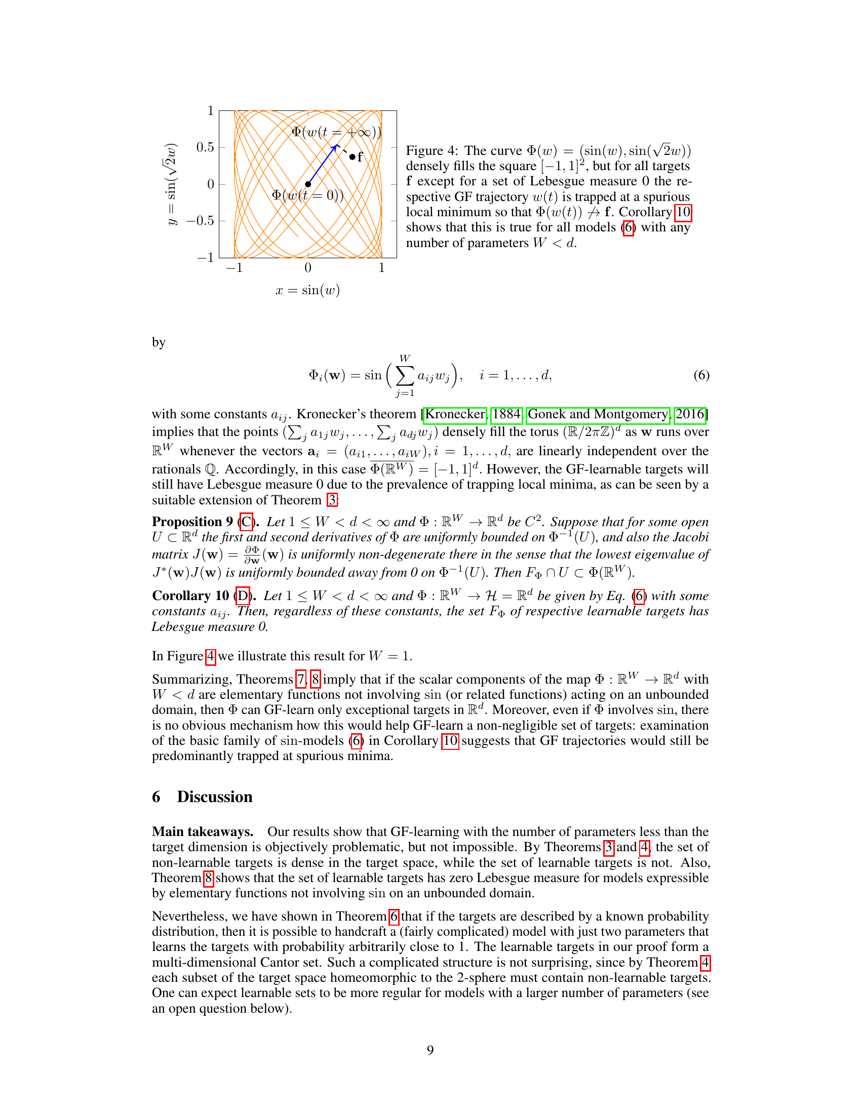
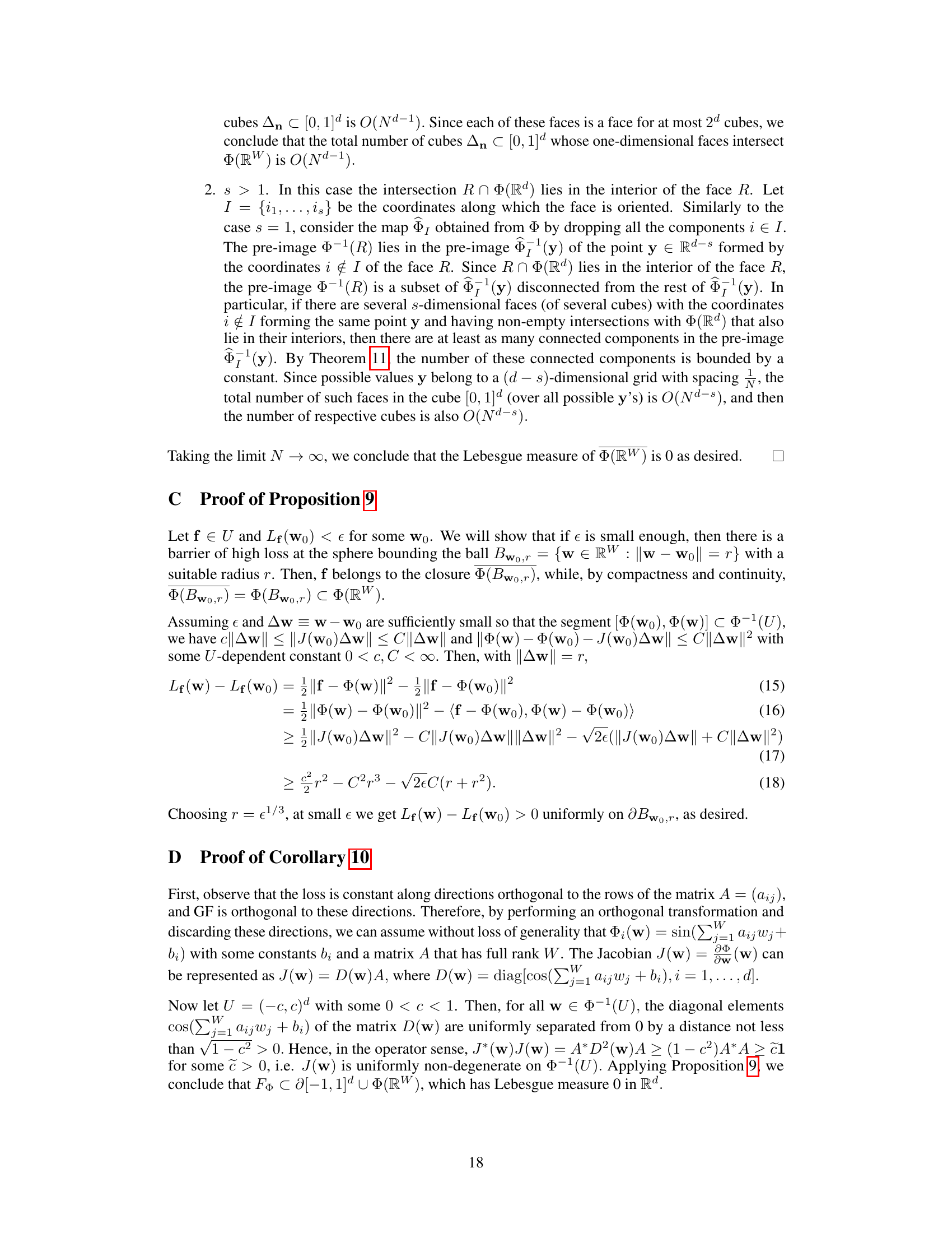
🔼 This figure shows a curve in a 2D space defined by the equations x = sin(w) and y = sin(√2w). The curve densely fills the [-1, 1] x [-1, 1] square. However, for almost all target points ‘f’ in the square, the gradient flow (GF) trajectory does not converge to ‘f’. Instead, the trajectory gets stuck at a local minimum, preventing convergence to the desired target. This illustrates that even when the model’s output densely covers the target space, underparameterization can severely limit the ability to learn the targets via gradient flow. Corollary 10 in the paper generalizes this behavior to higher dimensions.
read the caption
Figure 4: The curve Φ(w) = (sin(w), sin(√2w)) densely fills the square [-1,1]2, but for all targets f except for a set of Lebesgue measure 0 the respective GF trajectory w(t) is trapped at a spurious local minimum so that Φ(w(t)) → f. Corollary 10 shows that this is true for all models (6) with any number of parameters W < d.
Full paper#
