TL;DR#
Current research debates whether neural networks learn and implement algorithms or just use heuristics. This paper investigates this in the context of chess, focusing on the strong AI, Leela Zero. The challenge is understanding how such complex AIs work internally, and whether they utilize any advanced algorithms like look-ahead search.
The researchers used several interpretability techniques to study Leela Zero’s internal mechanisms. They analyzed activation patterns, attention heads, and trained a simple prediction probe. The results show clear evidence that Leela Zero has learned to use look-ahead, actively representing and using future optimal moves in its decision-making process. This contradicts the hypothesis that neural networks only rely on heuristics and demonstrates that they can learn and implement sophisticated algorithms. The findings have important implications for the interpretability and potential capabilities of neural networks.
Key Takeaways#
Why does it matter?#
This paper is crucial because it demonstrates that neural networks can learn complex algorithms like look-ahead, rather than simply relying on heuristics; this challenges our assumptions about how neural networks operate and opens doors for deeper mechanistic understanding of neural network capabilities and their potential for solving complex problems.
Visual Insights#
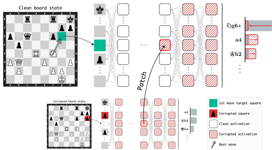
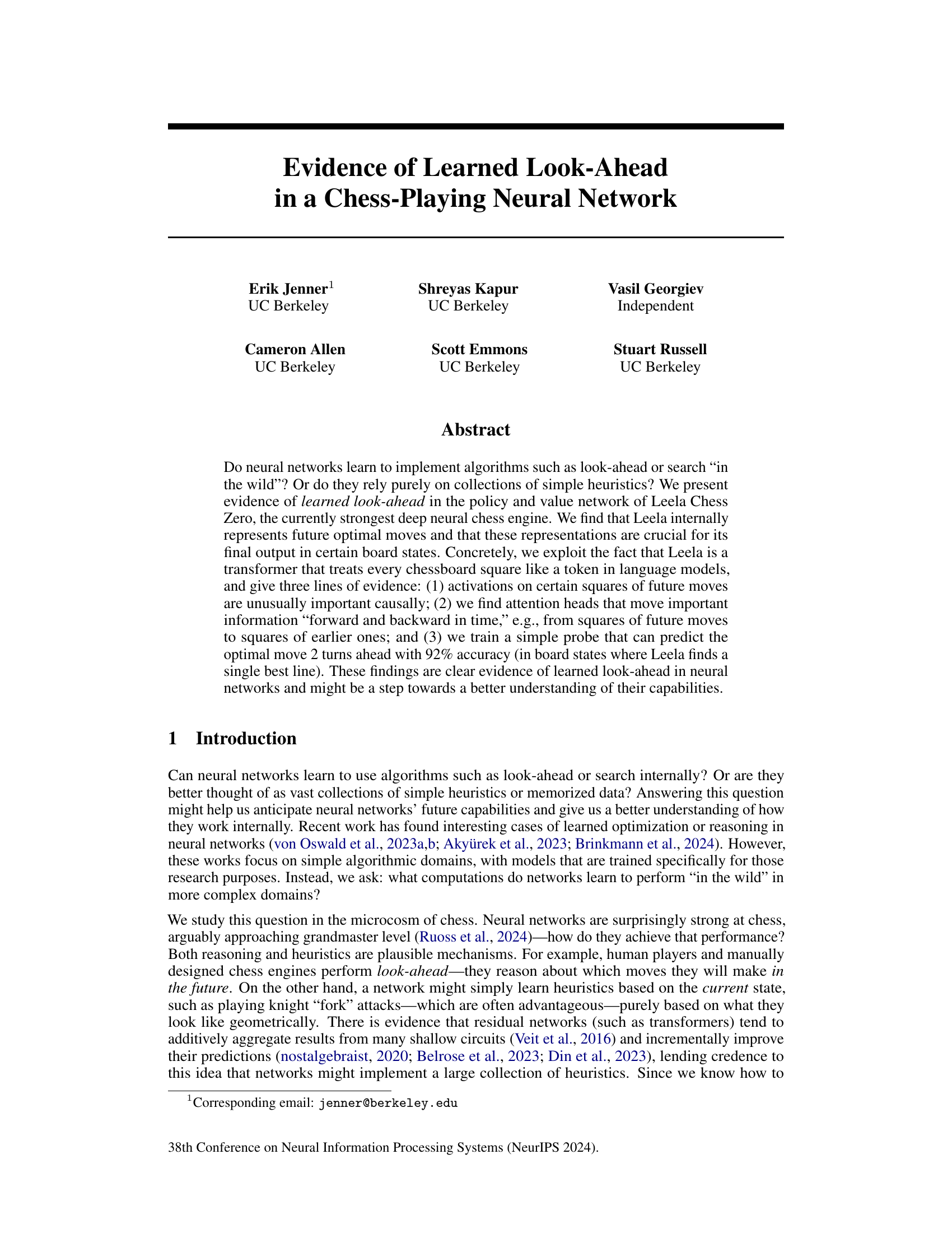
🔼 This figure demonstrates the activation patching technique used to investigate the importance of specific activations in Leela’s network. It shows a ‘clean’ board state and a ‘corrupted’ version of that state. By replacing activations from the corrupted state into the clean state’s forward pass, researchers can observe how the model’s output changes. This highlights which activations are crucial for accurate decision-making and reveals information storage within the network.
read the caption
Figure 1: Activation patching lets us study where important information is stored in Leela. Here, we patch an activation in one particular square and layer from the forward pass on a 'corrupted' board state (bottom) into the forward pass on a 'clean' state (top). Each row in the network corresponds to one chessboard square, which Leela treats like a token in a language model. The intervention drastically affects Leela's output (right), telling us that the activation on the patched square stores information necessary for Leela's performance in this state. Only patching on specific squares has significant effects. See https://leela-interp.github.io/ for more (animated) examples.
In-depth insights#
Learned Lookahead#
The concept of “Learned Lookahead” in the context of AI, specifically within the domain of game-playing neural networks, is a fascinating one. The research explores whether these networks, trained on vast amounts of game data, develop internal mechanisms that resemble algorithmic lookahead strategies, or if their success relies solely on sophisticated heuristics. The findings suggest a strong case for learned lookahead, demonstrating that the network develops internal representations of optimal future moves, rather than merely relying on pattern recognition from past games. This is supported by several key observations: causal analysis revealing the outsized importance of future move activations, attention mechanisms connecting earlier moves to the predicted consequences of later ones, and the successful prediction of optimal moves several steps ahead by a probe network. These results challenge the conventional understanding of how deep neural networks solve complex problems, indicating a potential for emergent algorithmic reasoning rather than mere pattern matching. While the precise mechanisms remain an open question, the research significantly advances our understanding of how neural networks might learn and use algorithms “in the wild” and opens up possibilities for further investigation into the nature of algorithmic reasoning in AI.
Activation Patching#
Activation patching is a powerful technique used to probe the causal influence of specific neural network components. By selectively replacing activations from one forward pass with those from another (e.g., a corrupted version of the input), researchers can isolate the contribution of a given component. This method is particularly valuable when studying complex models like those employed in games like chess, where traditional debugging methods are insufficient. The key insight lies in observing how downstream model behavior changes due to this localized intervention. Significant shifts indicate a crucial role for the altered component in reaching the model’s final decision, demonstrating causal, not merely correlational importance. While ingenious, the effectiveness of activation patching heavily relies on the choice of corruption. Carefully designed corruptions, perhaps derived using a simpler model to distinguish between consequential and superficial alterations, maximises the clarity and depth of the results. Thus, activation patching offers a powerful causal interpretation method that moves beyond simple correlation analyses, offering a valuable window into the intricate workings of complex neural networks.
Attention Heads#
The concept of ‘attention heads’ in the context of neural networks, particularly within the architecture of a chess-playing AI like Leela Chess Zero, is crucial for understanding how the model processes information and makes decisions. Attention heads act as mechanisms to weigh the importance of different parts of the input (in this case, different squares on a chessboard). The paper’s findings suggest that certain attention heads in Leela specifically focus on squares representing future moves in an optimal game sequence, highlighting the AI’s ability to perform a form of look-ahead. This is a significant finding because it implies that the network isn’t just relying on simple heuristics but is learning to internally represent and reason about future game states. Furthermore, the analysis shows attention heads can move information both forward and backward in time, suggesting a complex interplay of information flow within the network, enabling the AI to effectively consider short-term consequences of its actions. The ability of a simple probe to accurately predict future moves based on the activation patterns of these attention heads is strong evidence supporting the hypothesis of learned look-ahead. In essence, the investigation of attention heads in this research provides compelling evidence that neural networks in complex domains can learn sophisticated algorithms beyond simple pattern recognition.
Probe Accuracy#
The concept of “Probe Accuracy” in evaluating a model’s ability to predict future moves within a complex game like chess is crucial. The probes, simple bilinear models, were designed to assess whether the network internally represents future game states by leveraging activations from specific layers. High probe accuracy (92%) in predicting the optimal move two turns ahead provides strong evidence of learned look-ahead. This is not mere memorization; it signifies the model’s internal representation of future game states and the causal influence of those states on its immediate decisions. The success hinges on targeting specific activations linked to future moves, indicating that the network isn’t just relying on heuristics but employs a more sophisticated, algorithmic approach. This is particularly notable because the probe itself is simplistic; its effectiveness is entirely dependent on the network’s capacity to internally represent future information, underscoring the significance of the finding.
Chess AI Limits#
Discussions around “Chess AI Limits” would explore the boundaries of current chess AI capabilities. A key aspect would be the AI’s reliance on vast computational resources and massive datasets for training, highlighting the inherent scalability limitations. While AIs like AlphaZero and Leela Chess Zero demonstrate superhuman performance, their success is tied to specific algorithmic approaches and potentially lacks the adaptability and general intelligence of humans. The lack of explainability in AI decisions remains a considerable obstacle, impeding our understanding of their decision-making processes and making it difficult to identify and address potential weaknesses. Furthermore, analyzing the AI’s vulnerability to specific types of chess positions or strategies, such as those involving complex sacrifices or long-term strategic planning, would reveal blind spots and limitations. Examining whether current AI’s truly “understand” chess or merely excel through pattern recognition and statistical analysis is crucial to ascertain the true extent of their capabilities and future development prospects. This would ultimately reveal the gap between brute-force computation and true strategic understanding in the game of chess, leading to deeper insights into the nature of artificial intelligence itself.
More visual insights#
More on figures

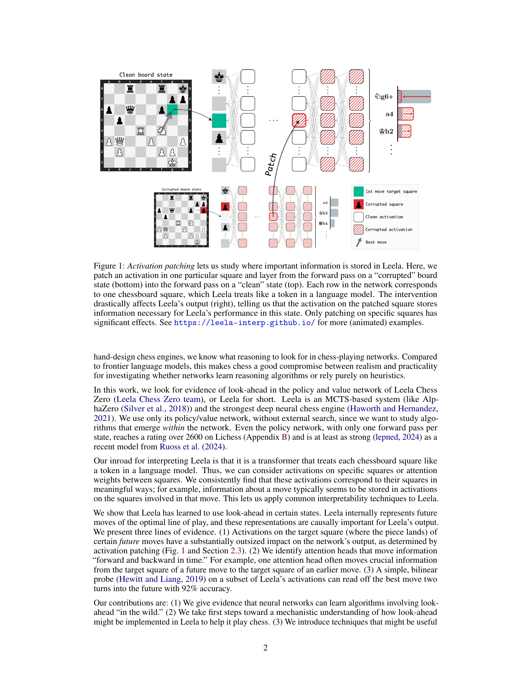
🔼 This figure shows an example of a chess puzzle used in the paper’s experiments. The top row illustrates the initial position, the position after the first move, and the position after the second move in the optimal sequence of moves. The optimal sequence consists of three moves to checkmate. The figure highlights the target squares of the first (green) and third (blue) moves of this sequence. The bottom row illustrates that Leela processes each board state separately to output a move probability distribution.
read the caption
Figure 2: Top row: An example of the puzzles we use. It is white's turn in the starting state, and the only winning action is to move the knight to g6. Black's only response is taking the knight with the pawn; then white checkmates by moving the rook to h4. We will see the colored squares again: the target square of the 1st move in this principal variation (green) and the target square of the 3rd move (blue). Below: Leela receives each state as a separate input and computes a policy in that state.
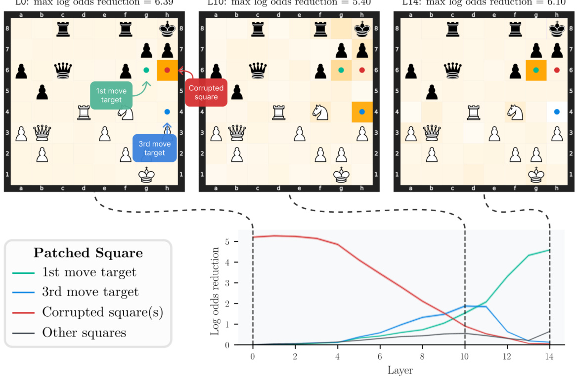
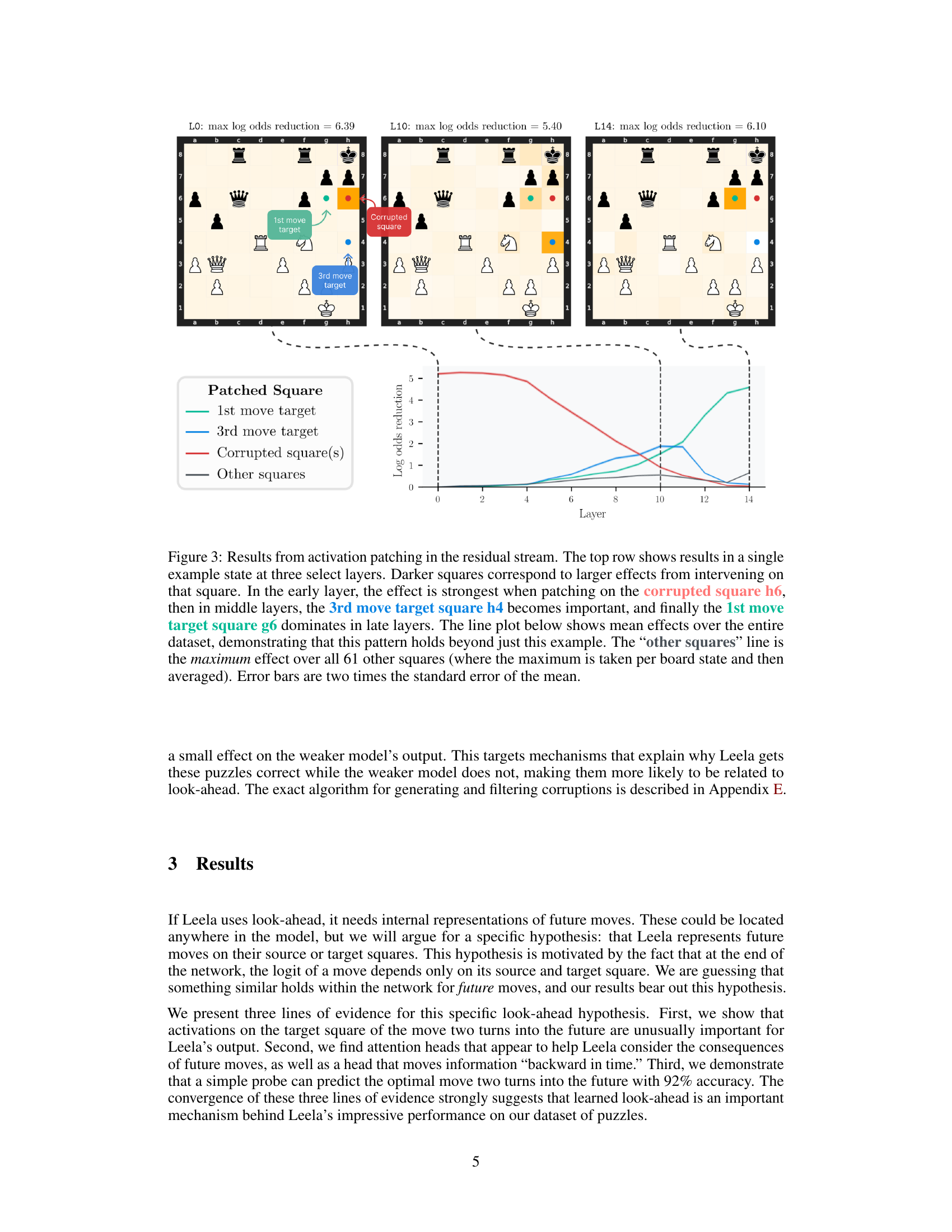
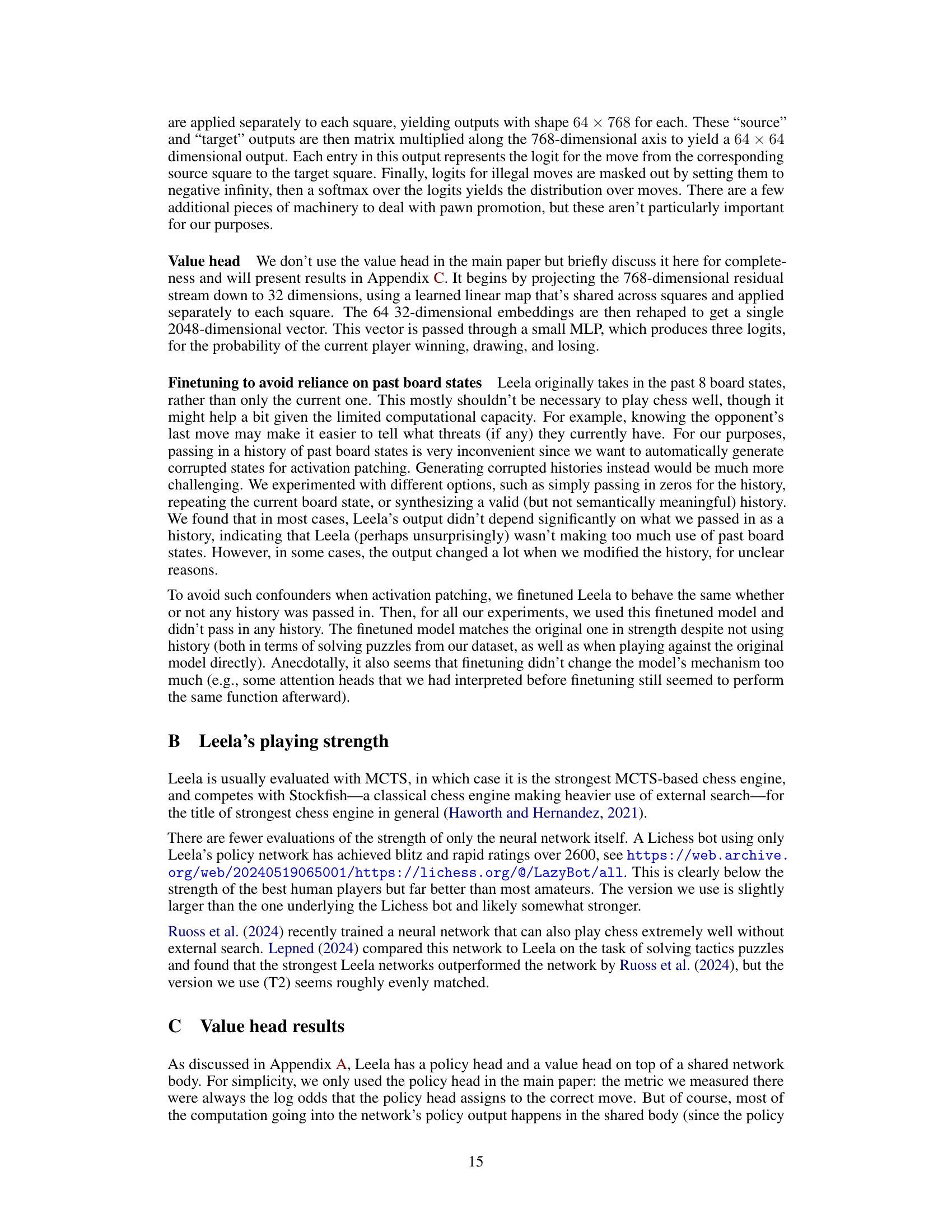
🔼 This figure shows the results of activation patching experiments on Leela’s residual stream. The top part illustrates how patching activations on specific squares affects Leela’s output in a single chess state across three different layers (L8, L10, L14). The color intensity of squares represents the magnitude of effect, showing how the importance of different squares varies across layers. The bottom line graph shows average effects across multiple board states, illustrating that patching the 3rd move target square (h4) has a significant impact in the middle layers, while the 1st move target (g6) is most influential in later layers. The ‘other squares’ line serves as a baseline comparison.
read the caption
Figure 3: Results from activation patching in the residual stream. The top row shows results in a single example state at three select layers. Darker squares correspond to larger effects from intervening on that square. In the early layer, the effect is strongest when patching on the corrupted square h6, then in middle layers, the 3rd move target square h4 becomes important, and finally the 1st move target square g6 dominates in late layers. The line plot below shows mean effects over the entire dataset, demonstrating that this pattern holds beyond just this example. The 'other squares' line is the maximum effect over all 61 other squares (where the maximum is taken per board state and then averaged). Error bars are two times the standard error of the mean.
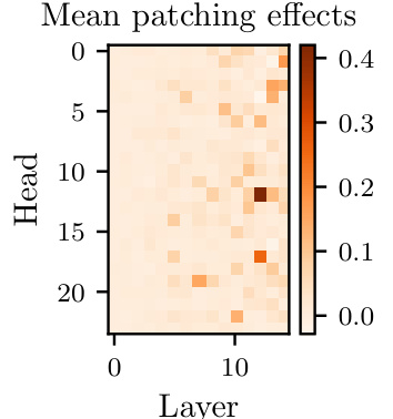
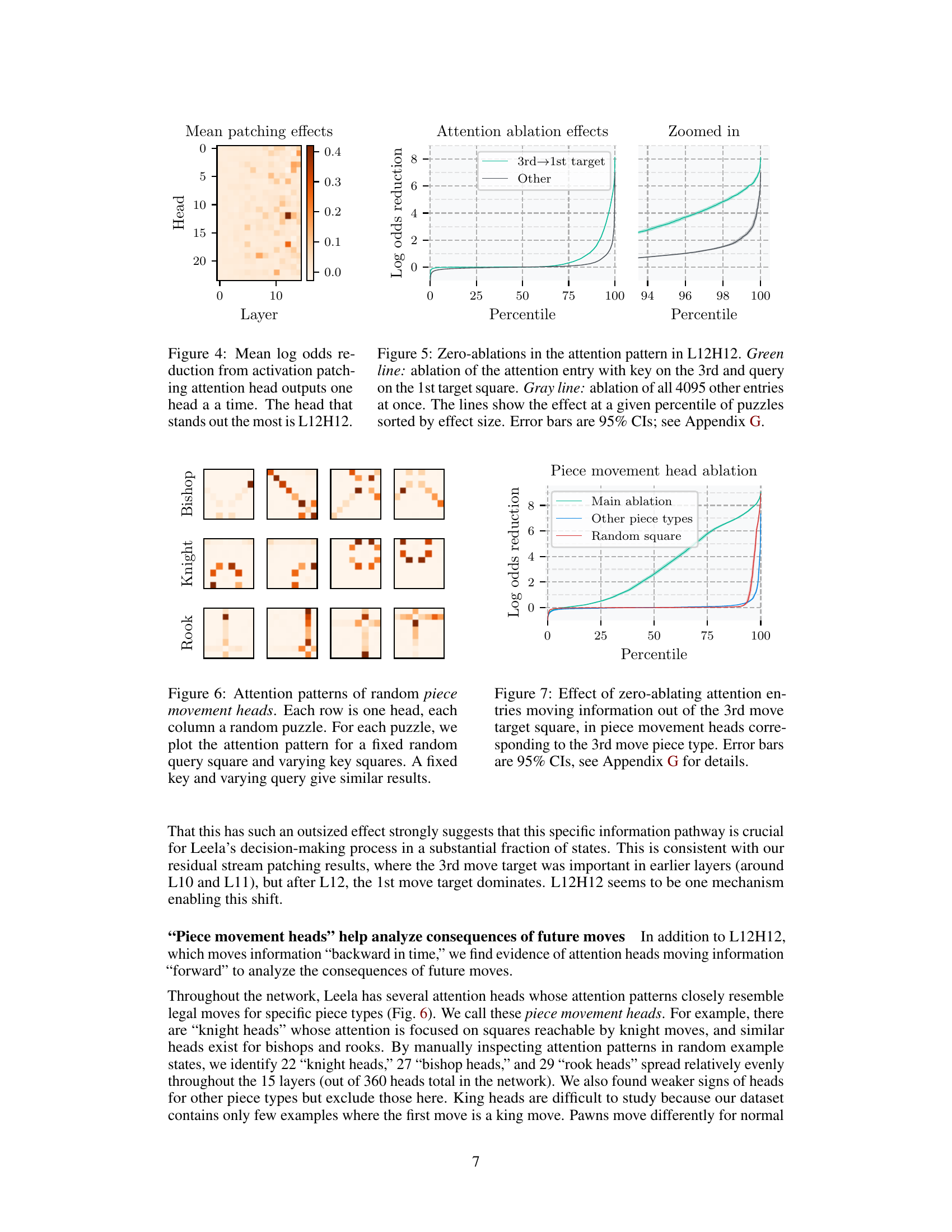
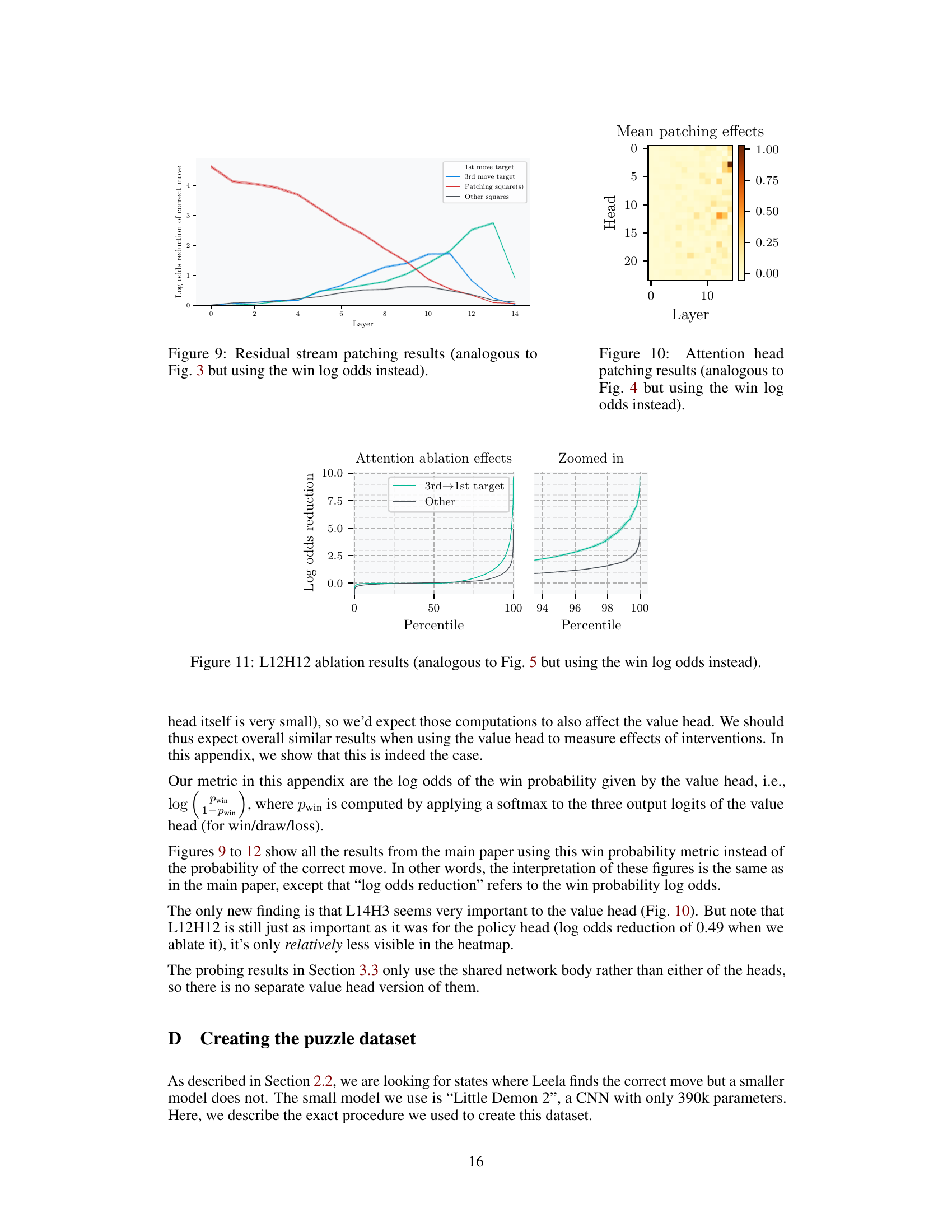
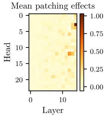
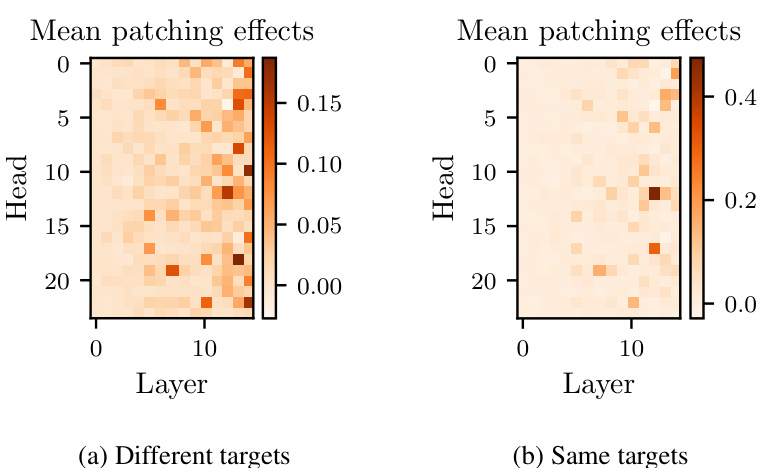
🔼 This figure shows the results of activation patching on attention heads in Leela’s network. Each cell in the heatmap represents the average effect on the log odds of the correct move when the outputs of a specific attention head are replaced with those from a corrupted board state. The color intensity indicates the magnitude of the effect, with darker colors indicating larger effects. The results show that one attention head (L12H12) stands out as having a much larger average effect than any other attention head.
read the caption
Figure 4: Mean log odds reduction from activation patching attention head outputs one head at a time. The head that stands out the most is L12H12.

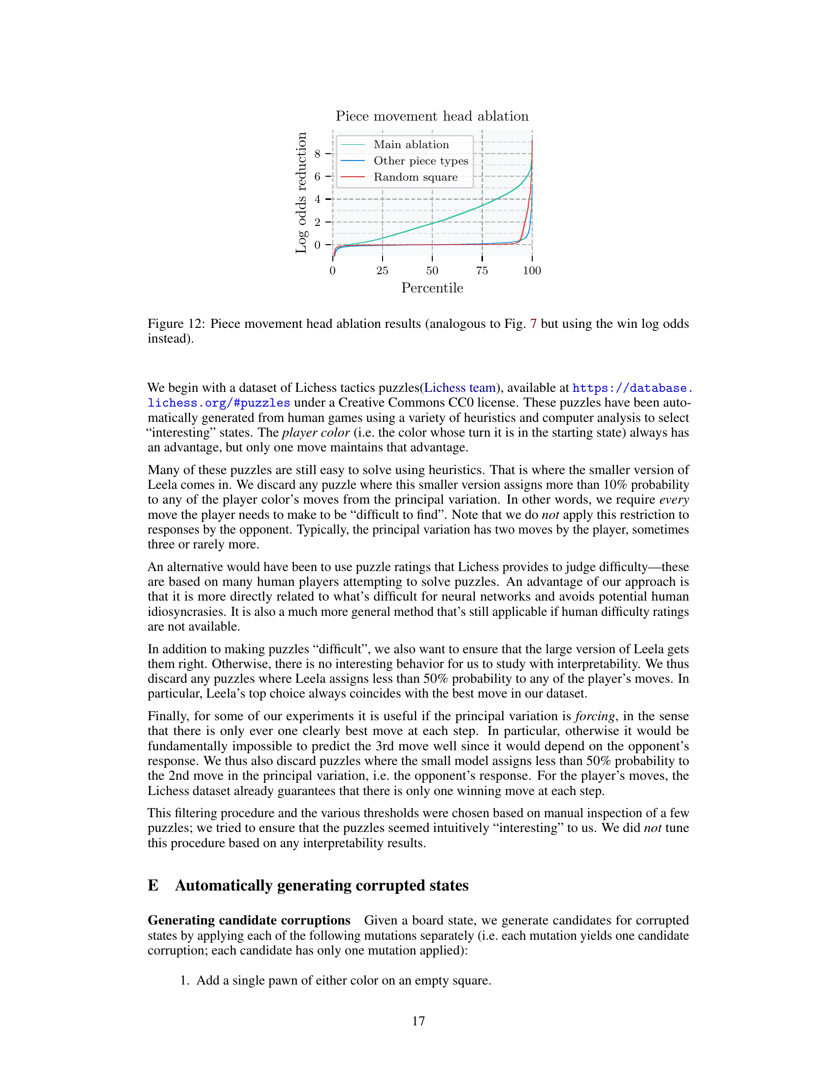
🔼 This figure shows the results of zeroing out specific attention entries in attention head L12H12. The green line represents the effect of removing only the attention entry where the key corresponds to the 3rd move target square and the query corresponds to the 1st move target square. The gray line shows the effect of removing all other attention entries simultaneously. The x-axis represents the percentile of puzzles sorted by the magnitude of the effect, and the y-axis represents the log odds reduction. The figure demonstrates that removing only the attention entry between the 1st and 3rd move target squares has a significantly larger effect than removing all other attention entries.
read the caption
Figure 5: Zero-ablations in the attention pattern in L12H12. Green line: ablation of the attention entry with key on the 3rd and query on the 1st target square. Gray line: ablation of all 4095 other entries at once. The lines show the effect at a given percentile of puzzles sorted by effect size. Error bars are 95% CIs; see Appendix G.
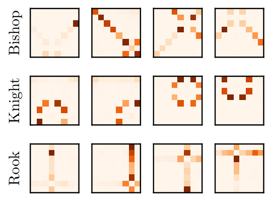
🔼 This figure shows the attention patterns of different heads in the Leela network. Each row represents a different attention head, and each column shows a different puzzle. The heatmaps visualize attention weights, indicating which key squares (target squares) are most attended to for a given query square (source square). Each head exhibits patterns consistent with specific piece movement types (knight, bishop, rook), suggesting that the network uses these heads to analyze the consequences of future moves involving those pieces.
read the caption
Figure 6: Attention patterns of random piece movement heads. Each row is one head, each column a random puzzle. For each puzzle, we plot the attention pattern for a fixed random query square and varying key squares. A fixed key and varying query give similar results.
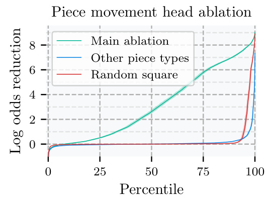
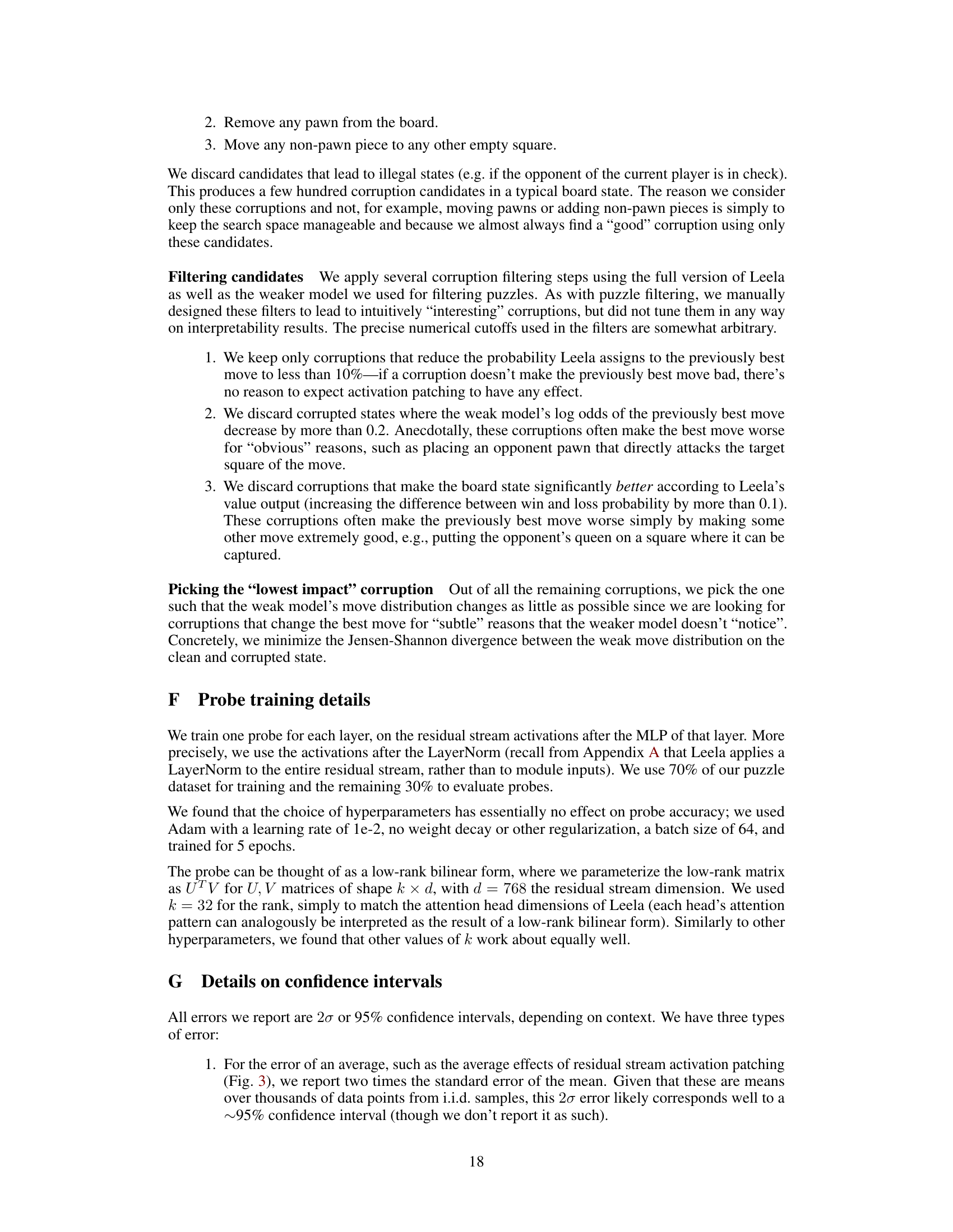
🔼 This figure shows the effect of removing (zeroing out) attention weights related to the third move’s target square in the attention heads focused on the type of piece that occupies that square. The main ablation line depicts the effect of zeroing out only the attention weights that relate the third move’s target square to other squares; the other piece types line shows the effect of zeroing out all such attention weights for piece types other than the one involved in the third move; the random square line depicts the average effect of ablating attention weights for random squares. The results demonstrate that removing information specifically from the third move’s target square in relevant piece-movement heads significantly impacts the model’s prediction accuracy.
read the caption
Figure 7: Effect of zero-ablating attention entries moving information out of the 3rd move target square, in piece movement heads corresponding to the 3rd move piece type. Error bars are 95% CIs, see Appendix G for details.
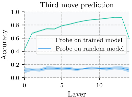
🔼 This figure shows the results of using a bilinear probe to predict the target square of the 3rd move in a chess game. The probe’s accuracy is plotted against the layer of the neural network from which the activations are taken. A comparison is made against a probe trained on a randomly initialized network to demonstrate that the results are not due to chance. The error bars combine the standard error of the mean across five separate training runs and the standard error of estimating the accuracy.
read the caption
Figure 8: Results of a bilinear probe for predicting the 3rd move target square. Errors combine standard errors of the mean for five probe training runs with standard errors for accuracy estimates; see Appendix G.
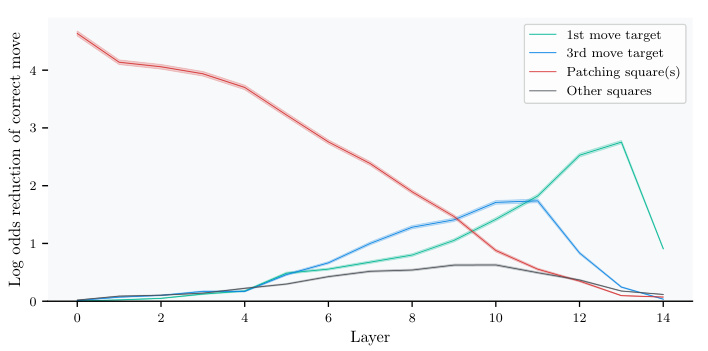
🔼 This figure shows the results of activation patching experiments on Leela’s residual stream. Activation patching is a technique used to determine the causal importance of specific model components by replacing their activations with those from a different forward pass. The experiment patches activations on different squares at three selected layers, observing how changes affect Leela’s output. The top row displays the results for a single state, while the line plot below shows the average effect across the entire dataset. The results demonstrate that the activations on specific squares (especially future move targets) are unusually important for Leela’s prediction accuracy, supporting the hypothesis that Leela uses look-ahead.
read the caption
Figure 3: Results from activation patching in the residual stream. The top row shows results in a single example state at three select layers. Darker squares correspond to larger effects from intervening on that square. In the early layer, the effect is strongest when patching on the corrupted square h6, then in middle layers, the 3rd move target square h4 becomes important, and finally the 1st move target square g6 dominates in late layers. The line plot below shows mean effects over the entire dataset, demonstrating that this pattern holds beyond just this example. The 'other squares' line is the maximum effect over all 61 other squares (where the maximum is taken per board state and then averaged). Error bars are two times the standard error of the mean.
🔼 This figure displays the results of activation patching experiments on Leela’s residual stream. The top panel shows a heatmap for three selected layers (1, 10, 14), illustrating the impact of patching activations on specific squares. Darker colors indicate a stronger causal effect on Leela’s output. The pattern shows a shift in importance from the corrupted square (h6) in the early layers to the 3rd move target square (h4) in the middle layers, and finally to the 1st move target square (g6) in the later layers. The bottom panel presents a line graph showing the average effect of patching on different squares across layers over the entire dataset, confirming this trend. The ‘other squares’ line represents the maximum effect observed for any of the remaining 61 squares in each board state.
read the caption
Figure 3: Results from activation patching in the residual stream. The top row shows results in a single example state at three select layers. Darker squares correspond to larger effects from intervening on that square. In the early layer, the effect is strongest when patching on the corrupted square h6, then in middle layers, the 3rd move target square h4 becomes important, and finally the 1st move target square g6 dominates in late layers. The line plot below shows mean effects over the entire dataset, demonstrating that this pattern holds beyond just this example. The 'other squares' line is the maximum effect over all 61 other squares (where the maximum is taken per board state and then averaged). Error bars are two times the standard error of the mean.
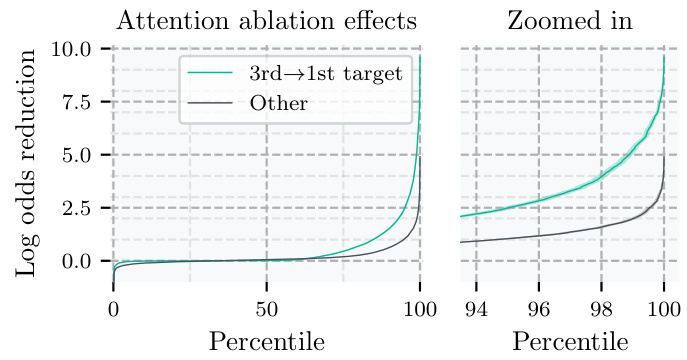
🔼 This figure shows the impact of ablating specific attention entries in head L12H12 of Leela’s network. The green line displays the effect of removing the attention entry where the key is the 3rd move target square and the query is the 1st move target square. The gray line shows the effect of removing all other entries simultaneously. The x-axis represents the percentile of puzzles sorted by the magnitude of the effect, and the y-axis represents the log odds reduction of the correct move. The plot demonstrates that ablating the single attention entry (green) has a much larger impact than ablating all other entries (gray), indicating the importance of this specific connection for Leela’s performance.
read the caption
Figure 5: Zero-ablations in the attention pattern in L12H12. Green line: ablation of the attention entry with key on the 3rd and query on the 1st target square. Gray line: ablation of all 4095 other entries at once. The lines show the effect at a given percentile of puzzles sorted by effect size. Error bars are 95% CIs; see Appendix G.
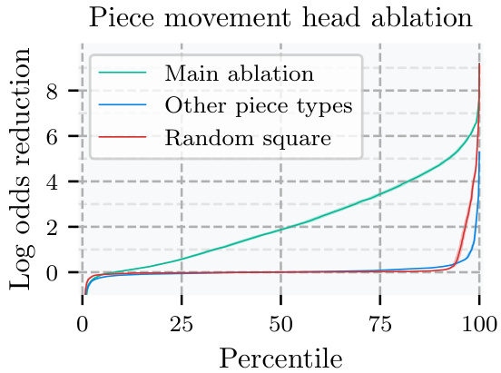
🔼 This figure shows the result of ablating attention entries that move information from the 3rd move target square in the ‘piece movement heads’. Piece movement heads are attention heads whose attention patterns resemble legal moves for specific chess piece types. The ablation specifically targets entries where the key is on the 3rd move target square, except for the entries between the source and target square of the 3rd move. The plot shows the effect on log odds of the correct move against the percentile of the dataset sorted by effect size. This analysis reveals that zeroing out these specific attention entries significantly impacts the model’s predictions, suggesting that these pathways are crucial for analyzing the consequences of future moves.
read the caption
Figure 7: Effect of zero-ablating attention entries moving information out of the 3rd move target square, in piece movement heads corresponding to the 3rd move piece type. Error bars are 95% CIs, see Appendix G for details.

🔼 This figure displays the results of activation patching on Leela’s residual stream. The top panel shows activation patching results for a single chessboard state at three different layers (layers 3, 10, and 14). Darker colors represent larger effects from patching the activation on that square. The bottom panel shows the average effects across the whole dataset. The results demonstrate that activations on the target square of the third move have a disproportionately large effect on the network’s output, highlighting the importance of these future move representations for Leela’s performance.
read the caption
Figure 3: Results from activation patching in the residual stream. The top row shows results in a single example state at three select layers. Darker squares correspond to larger effects from intervening on that square. In the early layer, the effect is strongest when patching on the corrupted square h6, then in middle layers, the 3rd move target square h4 becomes important, and finally the 1st move target square g6 dominates in late layers. The line plot below shows mean effects over the entire dataset, demonstrating that this pattern holds beyond just this example. The 'other squares' line is the maximum effect over all 61 other squares (where the maximum is taken per board state and then averaged). Error bars are two times the standard error of the mean.
🔼 This figure shows the results of activation patching on Leela’s residual stream. Activation patching is a technique to measure the causal importance of specific model components by replacing their activations with those from a different forward pass. The top row shows the effects of patching activations at different layers (L10, L14) in a single example chess state. Darker squares indicate a greater effect on Leela’s output when those activations are patched. The pattern shows that the importance of certain squares changes across layers, with the 3rd move’s target square (h4) becoming increasingly important in the middle layers before the 1st move’s target square (g6) dominates in the later layers. The bottom line plot demonstrates that this trend generalizes across the entire dataset of chess puzzles, indicating the causal importance of target squares of future moves in Leela’s decisions.
read the caption
Figure 3: Results from activation patching in the residual stream. The top row shows results in a single example state at three select layers. Darker squares correspond to larger effects from intervening on that square. In the early layer, the effect is strongest when patching on the corrupted square h6, then in middle layers, the 3rd move target square h4 becomes important, and finally the 1st move target square g6 dominates in late layers. The line plot below shows mean effects over the entire dataset, demonstrating that this pattern holds beyond just this example. The 'other squares' line is the maximum effect over all 61 other squares (where the maximum is taken per board state and then averaged). Error bars are two times the standard error of the mean.

🔼 This figure shows the results of ablating the attention entry of L12H12 that moves information from the 3rd move target to the 1st move target. The green line shows the effect of ablating only that specific entry, while the grey line shows the effect of ablating all other attention entries in L12H12. The zoomed-in portion highlights the difference between the effects of these two ablations. The results are shown separately for puzzles where the 1st and 2nd move targets are the same (b) and those where they are different (a). The x-axis represents the percentile of puzzles ordered by effect size, and the y-axis shows the change in log-odds of the correct move due to the ablation.
read the caption
Figure 11: L12H12 ablation results (analogous to Fig. 5 but using the win log odds instead).
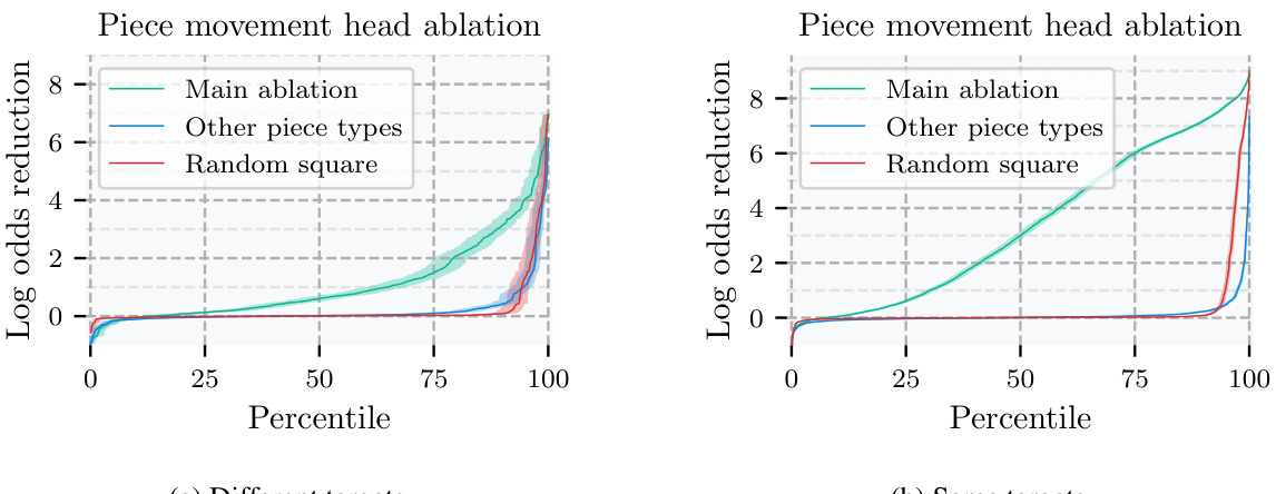
🔼 This figure shows the effect of ablating attention entries that move information out of the 3rd move target square in the piece movement heads. The ablations are performed separately for each puzzle and are split into two groups based on whether the 1st and 2nd move target squares are the same or different. The results show that for each puzzle, the largest reduction in log odds is usually larger when the 1st and 2nd move target squares are the same.
read the caption
Figure 16: Ablations in piece movement heads, analogous to Fig. 7.
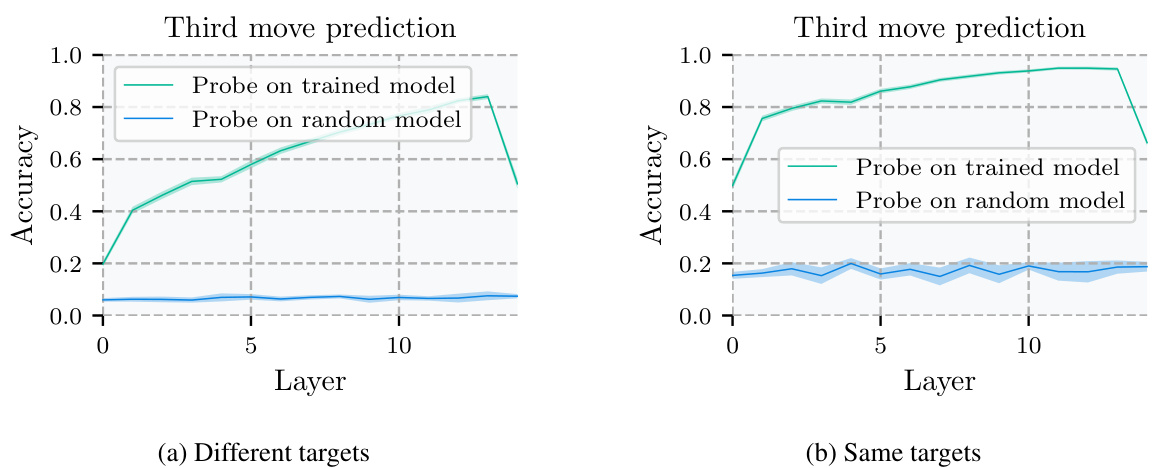
🔼 This figure shows the results of a bilinear probe trained to predict the 3rd move target square in chess puzzles. The probe’s accuracy increases with the network layer depth, reaching a peak of approximately 92% accuracy after layer 12. In contrast, a probe trained on a randomly initialized network achieves significantly lower accuracy. The figure includes two subplots, one for puzzles where the 1st and 2nd move target squares differ, and one where they are the same.
read the caption
Figure 8: Results of a bilinear probe for predicting the 3rd move target square. Errors combine standard errors of the mean for five probe training runs with standard errors for accuracy estimates; see Appendix G.
Full paper#
