TL;DR#
Auto-labeling is a cost-effective way to create labeled datasets for machine learning but suffers from overconfident model predictions, reducing accuracy. Existing calibration methods haven’t fully solved this, limiting the effectiveness of threshold-based auto-labeling (TBAL). The core challenge lies in the inherent tension between maximizing coverage (auto-labeling more data) and maintaining a low error rate.
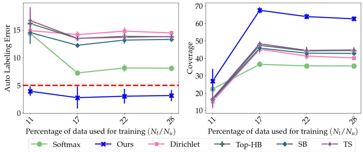
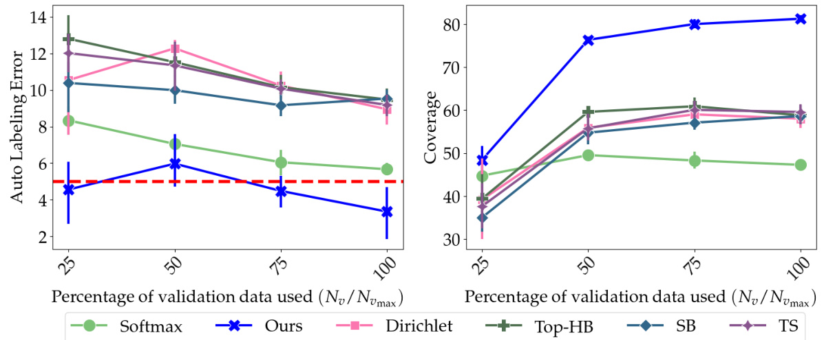
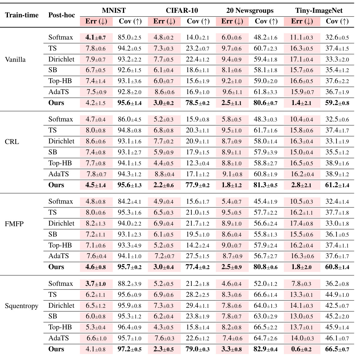
This paper introduces Colander, a novel framework that learns optimal confidence functions to maximize TBAL’s performance. Colander achieves significant improvements, boosting coverage by up to 60% while maintaining an error level below 5%. The method uses a practical approach, leveraging empirical estimates and optimizing surrogates to address the challenges of learning optimal confidence functions. Colander’s effectiveness is demonstrated through extensive evaluations on various datasets and models, highlighting its superior performance compared to standard calibration and alternative TBAL methods.
Key Takeaways#
Why does it matter?#
This paper is crucial for researchers in machine learning and data labeling. It directly addresses the high cost and time consumption associated with obtaining labeled data, a significant bottleneck in many ML projects. By proposing a novel, efficient auto-labeling method called Colander, which outperforms existing approaches, the paper offers a practical solution to a pervasive problem. This work opens up several avenues for further research, including exploring more sophisticated confidence functions and optimizing the integration of auto-labeling with active learning strategies. The results have direct implications for various industry applications and help advance the practical use of auto-labeling in real-world scenarios.
Visual Insights#

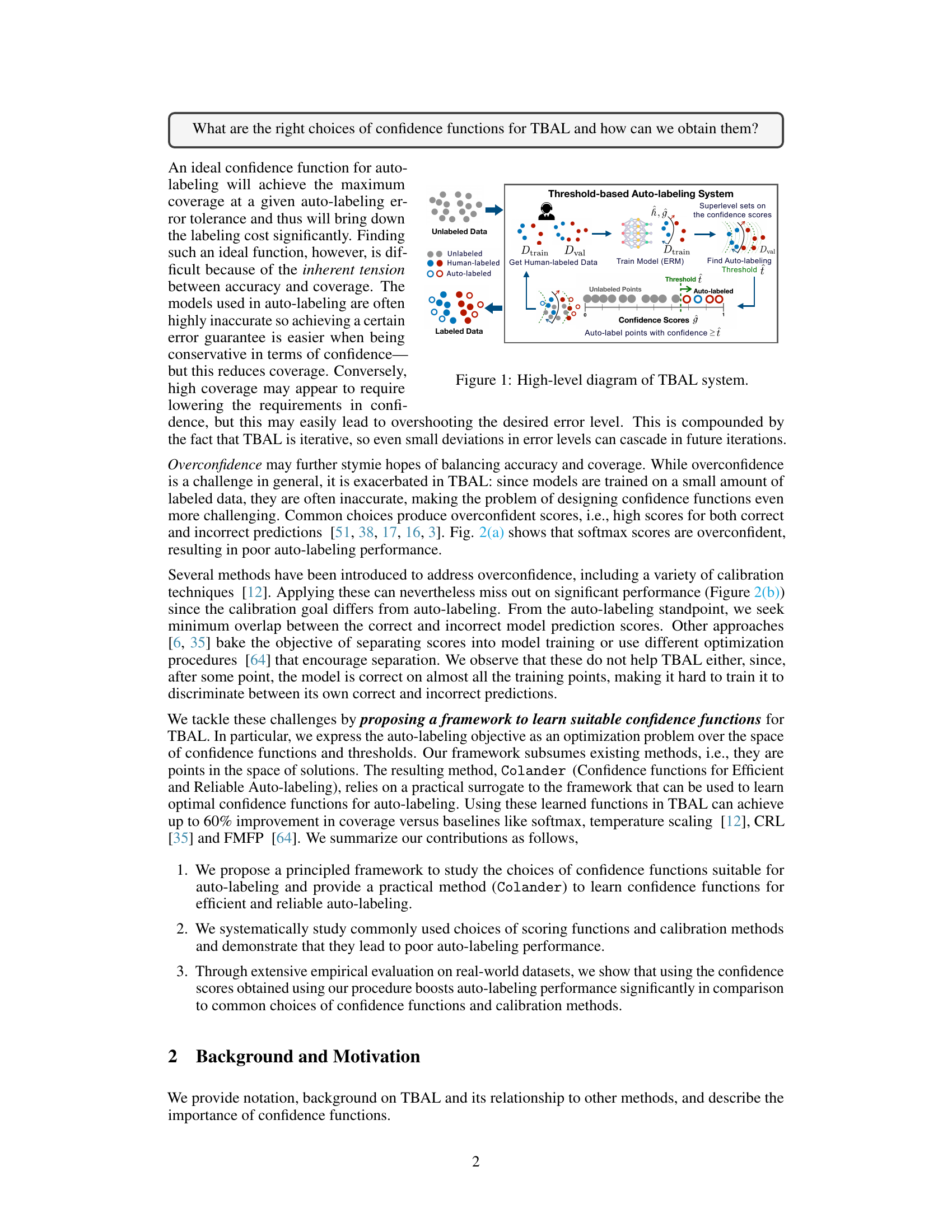
🔼 This figure illustrates the overall workflow of a Threshold-based Auto-labeling (TBAL) system. It begins with unlabeled data. A subset of this data is labeled by humans, used to train a model, and then a threshold is determined based on model confidence scores. Points above this threshold are automatically labeled by the model, augmenting the labeled dataset. The process iterates, querying more human labels and auto-labeling more points until the desired level of labeled data is achieved.
read the caption
Figure 1: High-level diagram of TBAL system.

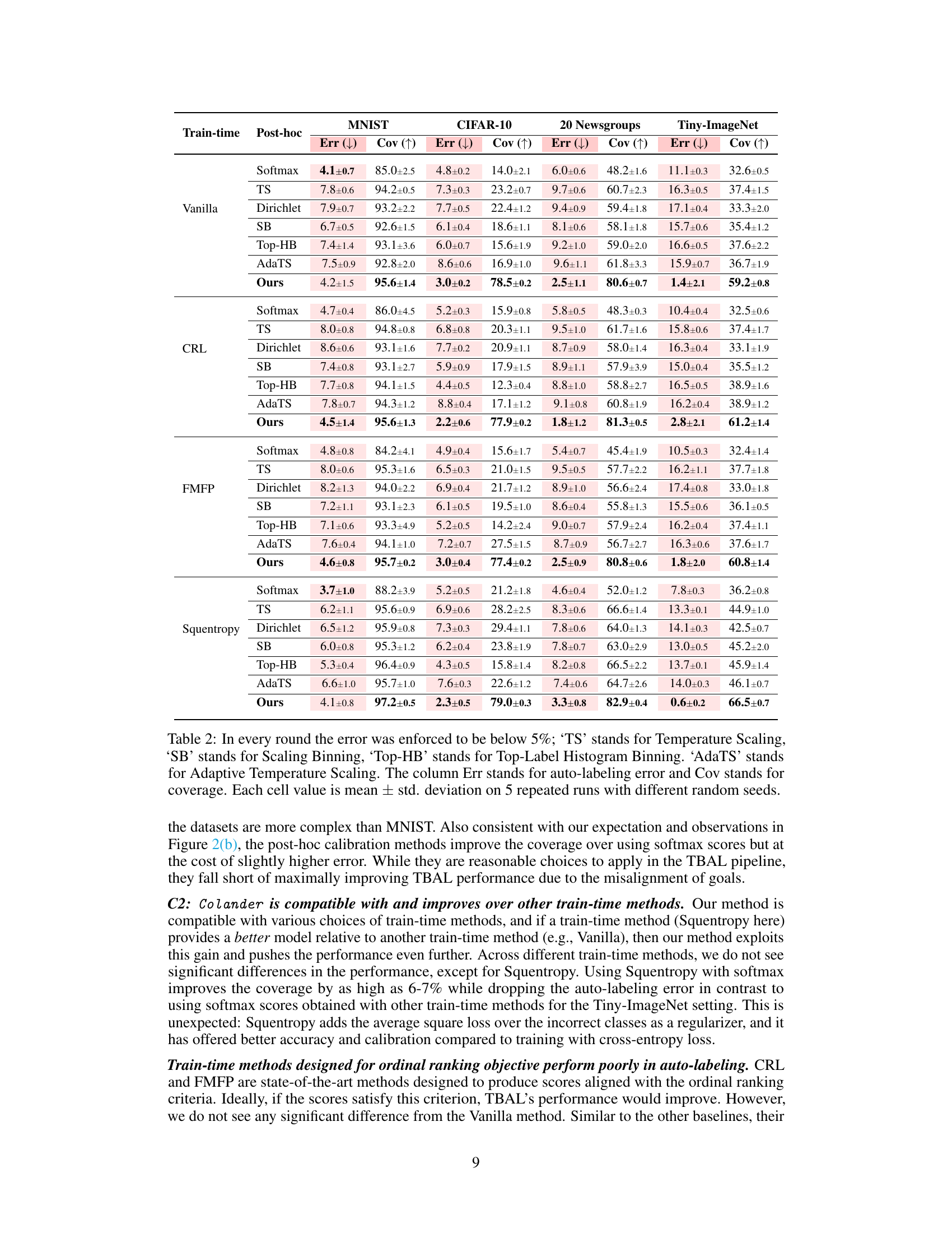
🔼 This table presents the performance comparison of different train-time and post-hoc methods for auto-labeling on four datasets: MNIST, CIFAR-10, 20 Newsgroup, and Tiny-Imagenet. For each dataset and method, the auto-labeling error and coverage are reported. The results are averaged over five repeated runs with different random seeds to ensure reliability. Temperature scaling, scaling binning, top-label histogram binning, and adaptive temperature scaling methods are included for comparison.
read the caption
Table 2: In every round the error was enforced to be below 5%; ‘TS’ stands for Temperature Scaling, ‘SB’ stands for Scaling Binning, ‘Top-HB’ stands for Top-Label Histogram Binning. ‘AdaTS’ stands for Adaptive Temperature Scaling. The column Err stands for auto-labeling error and Cov stands for coverage. Each cell value is mean ± std. deviation on 5 repeated runs with different random seeds.
In-depth insights#
TBAL Optimization#
TBAL (Threshold-Based Auto-Labeling) optimization focuses on improving the efficiency and accuracy of automatically labeling data. A core challenge is finding the optimal balance between maximizing the coverage (proportion of data automatically labeled) and minimizing the auto-labeling error. Effective optimization strategies often involve carefully selecting a confidence function, which determines which predictions are considered reliable enough for automatic labeling. The paper explores frameworks for finding optimal confidence functions, moving beyond simplistic approaches like using softmax outputs directly. A key insight is that the ideal confidence function isn’t simply about well-calibrated probabilities; it’s about maximizing the separation between correct and incorrect predictions. This is achieved by formulating the optimization as a balance between coverage and error. The proposed method, Colander, employs a practical surrogate to efficiently learn an optimal confidence function within this framework, significantly improving TBAL performance and achieving substantial gains over baselines. The method’s flexibility in handling various train-time procedures highlights its generalizability and usefulness in diverse settings.
Colander Method#
The Colander method, as described in the research paper, presents a novel approach to optimize confidence functions for threshold-based auto-labeling (TBAL). It addresses the limitations of existing methods that often produce overconfident scores, leading to suboptimal TBAL performance. The core of Colander involves a principled framework for studying optimal confidence functions, moving beyond ad-hoc choices. Instead of relying on off-the-shelf calibration techniques, Colander directly formulates the auto-labeling objective as an optimization problem, aiming to maximize coverage while maintaining a desired error level. A practical method is presented to learn optimal confidence functions using empirical estimates and differentiable surrogates. The resulting confidence functions, obtained through a tractable optimization process, are then integrated into the TBAL workflow to achieve significantly improved coverage while maintaining low error rates. The empirical evaluation demonstrates substantial improvements over baseline methods, highlighting the effectiveness of Colander in enhancing the efficiency and reliability of auto-labeling systems. This framework is particularly relevant because it provides a systematic, theoretically grounded approach to a critical component of TBAL.
Empirical Results#
The empirical results section would ideally present a thorough evaluation demonstrating the effectiveness of the proposed Colander method. This would involve comparing its performance against established baselines across multiple datasets, using metrics such as coverage and auto-labeling error. Key aspects to highlight would be the consistent improvements shown by Colander in achieving higher coverage while maintaining error levels below a predefined threshold. The analysis should also explore the impact of various hyperparameters and their optimization strategies. Visualizations, such as plots showcasing coverage and error across different methods, datasets, and training data budget sizes would help in understanding the trends and relative performance. A detailed discussion would be necessary to interpret the results, providing insights into why Colander surpasses the baselines. This might involve analyzing the behavior of different confidence functions under different conditions and explaining any unexpected outcomes. Finally, statistical significance must be carefully considered and clearly stated in the results, ensuring the observed improvements are not merely due to chance.
Future Work#
Future research directions stemming from this work on improved confidence functions for auto-labeling could explore several promising avenues. Extending the Colander framework to handle noisy labels is crucial for real-world applicability, as human annotations are often imperfect. Investigating alternative confidence function families beyond neural networks, such as those based on ensembles or Bayesian methods, could potentially yield further improvements in accuracy and coverage. A deeper theoretical analysis of the Colander optimization problem is needed to provide a stronger understanding of its convergence properties and limitations. Finally, evaluating the generalizability of Colander across a wider range of datasets and tasks is essential to demonstrate its robustness and broad applicability, establishing its potential as a valuable tool for various machine learning applications that rely on efficient and accurate data labeling.
Method Limits#
A hypothetical ‘Method Limits’ section for a research paper on auto-labeling would explore inherent constraints. Data scarcity is a primary limitation; auto-labeling heavily relies on limited labeled data, impacting model accuracy and generalization. The effectiveness hinges on the quality of the initial model, which might not be robust against overconfidence, noisy data, or domain shifts. Computational cost becomes significant as the dataset size increases; training and optimizing the model with post-hoc calibration methods can be computationally expensive. The proposed framework’s reliance on empirical estimates introduces another limitation; approximations could lead to sub-optimal solutions and affect the overall performance. Finally, the choice of confidence function impacts performance, necessitating a careful selection and optimization process. Exploring these limits can help refine the methodology and improve auto-labeling performance.
More visual insights#
More on figures

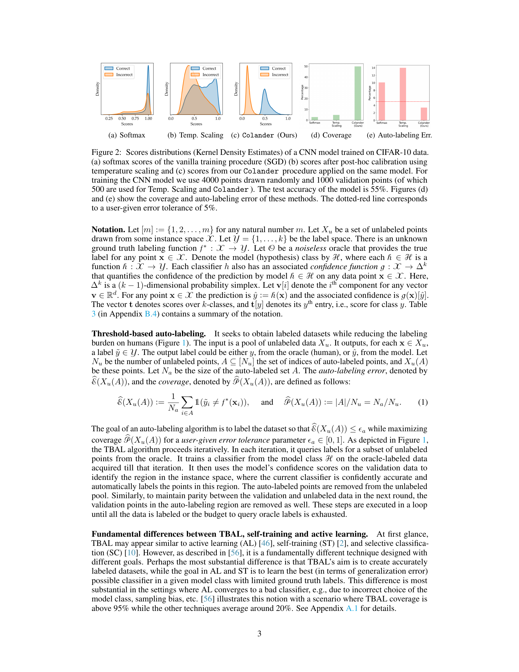
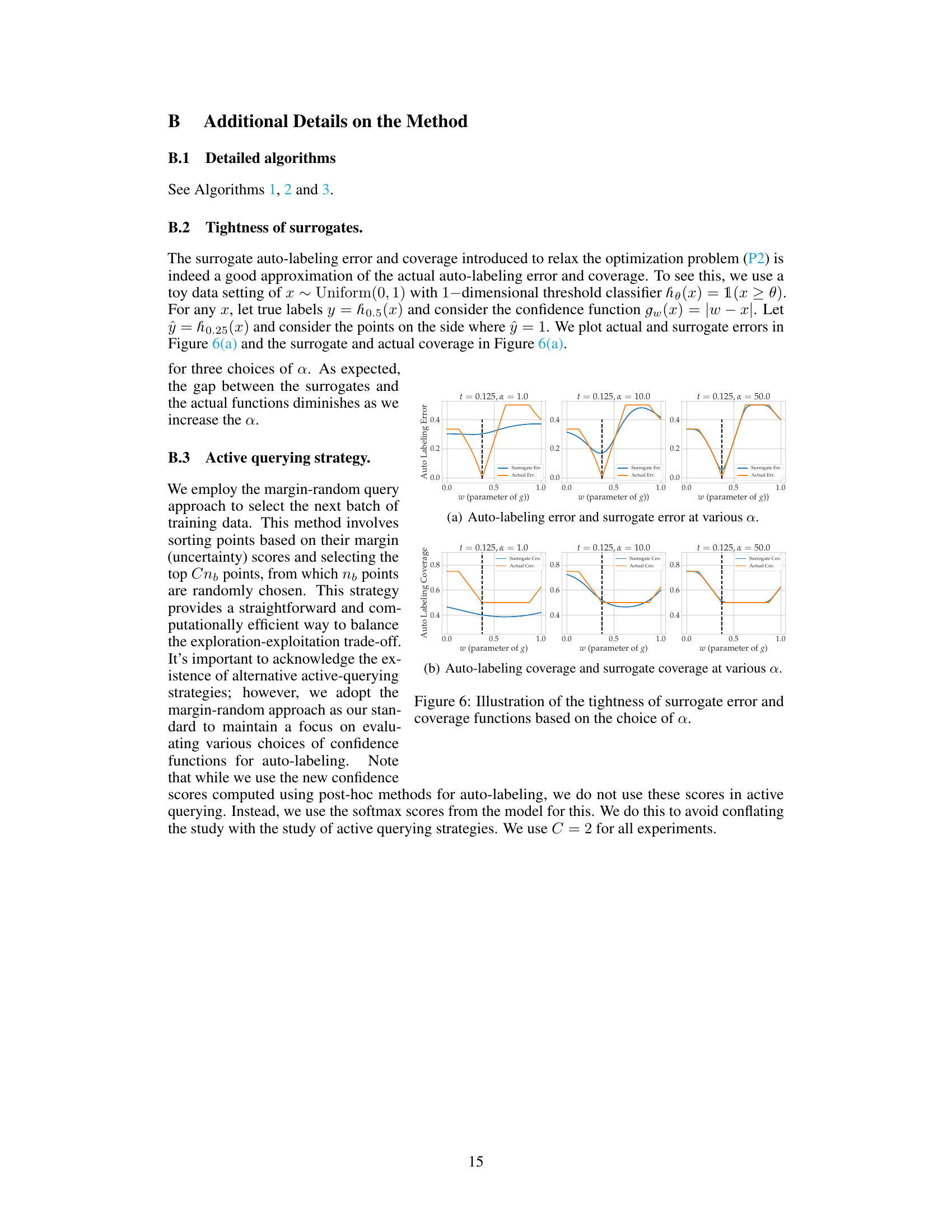
🔼 This figure shows the distribution of confidence scores from a CNN model trained on CIFAR-10 for correct and incorrect predictions, using three different methods: softmax, temperature scaling, and the proposed Colander method. It also shows the coverage and auto-labeling error for each method, highlighting Colander’s improved performance in balancing accuracy and coverage.
read the caption
Figure 2: Scores distributions (Kernel Density Estimates) of a CNN model trained on CIFAR-10 data. (a) softmax scores of the vanilla training procedure (SGD) (b) scores after post-hoc calibration using temperature scaling and (c) scores from our Colander procedure applied on the same model. For training the CNN model we use 4000 points drawn randomly and 1000 validation points (of which 500 are used for Temp. Scaling and Colander). The test accuracy of the model is 55%. Figures (d) and (e) show the coverage and auto-labeling error of these methods. The dotted-red line corresponds to a user-given error tolerance of 5%.

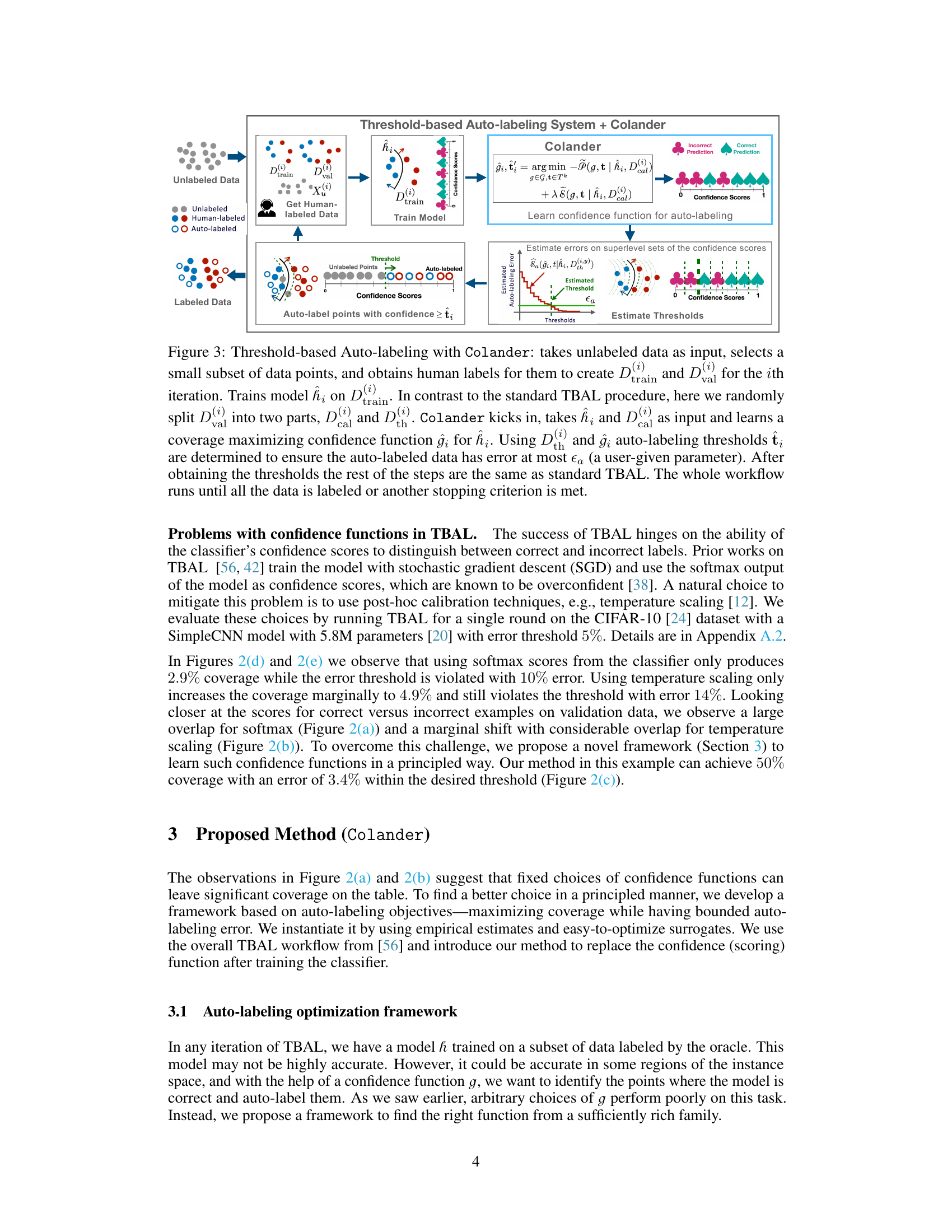
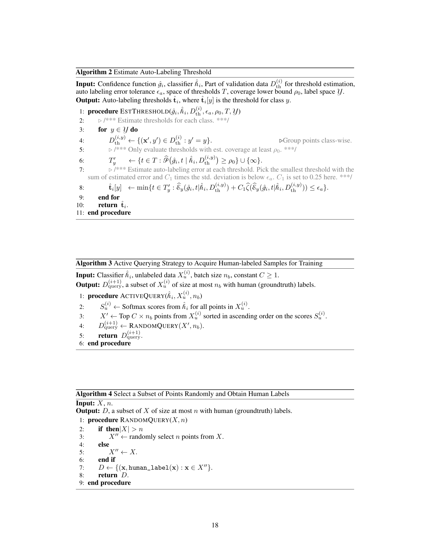
🔼 This figure illustrates the workflow of the proposed method, Colander, integrated into a threshold-based auto-labeling system. It shows how Colander learns a new confidence function to maximize coverage while maintaining a desired error rate. The iterative process involves training a model, using Colander to optimize the confidence function, estimating thresholds, and auto-labeling data points above the threshold. This continues until all data is labeled or a stopping criterion is met.
read the caption
Figure 3: Threshold-based Auto-labeling with Colander: takes unlabeled data as input, selects a small subset Dtrain(i) and Dval(i) of data points, and obtains human labels for them to create Dtrain(i) and Dval(i), for the ith iteration. Trains model hi on Dtrain(i). In contrast to the standard TBAL procedure, here we randomly split Dval(i) into two parts, Dcal(i) and Dth(i). Colander kicks in, takes hi and Dcal(i) as input and learns a coverage maximizing confidence function ĝi for hi. Using Dth(i) and ĝi auto-labeling thresholds ti are determined to ensure the auto-labeled data has error at most ea (a user-given parameter). After obtaining the thresholds the rest of the steps are the same as standard TBAL. The whole workflow runs until all the data is labeled or another stopping criterion is met.
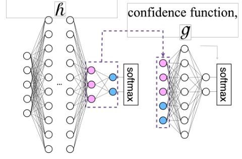
🔼 This figure illustrates the architecture of the confidence function g used in the Colander method. It shows a neural network that takes as input the concatenated outputs from the second-to-last and last layers of the classification model h. This concatenated input then passes through two fully connected layers (with tanh activation function) and finally a softmax layer to produce k confidence scores. The dashed purple boxes highlight the two fully connected layers of the g network.
read the caption
Figure 4: Our choice of g function.

🔼 This figure compares the score distributions obtained from three different methods: vanilla softmax, temperature scaling, and the proposed Colander method. It shows that Colander produces a better separation between correct and incorrect predictions, leading to improved coverage and reduced error in the auto-labeling process. The test accuracy of the underlying model is also provided for context.
read the caption
Figure 2: Scores distributions (Kernel Density Estimates) of a CNN model trained on CIFAR-10 data. (a) softmax scores of the vanilla training procedure (SGD) (b) scores after post-hoc calibration using temperature scaling and (c) scores from our Colander procedure applied on the same model. For training the CNN model we use 4000 points drawn randomly and 1000 validation points (of which 500 are used for Temp. Scaling and Colander). The test accuracy of the model is 55%. Figures (d) and (e) show the coverage and auto-labeling error of these methods. The dotted-red line corresponds to a user-given error tolerance of 5%.

🔼 This figure compares the score distributions of a CNN model trained on CIFAR-10 dataset using different methods: vanilla training with softmax scores, temperature scaling for calibration, and the proposed Colander method. It shows that Colander produces less overlapping scores between correct and incorrect predictions compared to softmax and temperature scaling, leading to improved performance in auto-labeling.
read the caption
Figure 2: Scores distributions (Kernel Density Estimates) of a CNN model trained on CIFAR-10 data. (a) softmax scores of the vanilla training procedure (SGD) (b) scores after post-hoc calibration using temperature scaling and (c) scores from our Colander procedure applied on the same model. For training the CNN model we use 4000 points drawn randomly and 1000 validation points (of which 500 are used for Temp. Scaling and Colander). The test accuracy of the model is 55%. Figures (d) and (e) show the coverage and auto-labeling error of these methods. The dotted-red line corresponds to a user-given error tolerance of 5%.

🔼 This figure shows the kernel density estimates of the confidence scores generated by three different methods: softmax, temperature scaling and the proposed Colander method. It highlights the overconfidence issue present in softmax scores, the limited improvement offered by temperature scaling, and the superior performance achieved by Colander in terms of both coverage and error rate.
read the caption
Figure 2: Scores distributions (Kernel Density Estimates) of a CNN model trained on CIFAR-10 data. (a) softmax scores of the vanilla training procedure (SGD) (b) scores after post-hoc calibration using temperature scaling and (c) scores from our Colander procedure applied on the same model. For training the CNN model we use 4000 points drawn randomly and 1000 validation points (of which 500 are used for Temp. Scaling and Colander). The test accuracy of the model is 55%. Figures (d) and (e) show the coverage and auto-labeling error of these methods. The dotted-red line corresponds to a user-given error tolerance of 5%.

🔼 This figure compares the score distributions of a CNN model trained on CIFAR-10 dataset using three different methods: vanilla training with softmax scores, temperature scaling for calibration, and the proposed Colander method. It visually demonstrates the overconfidence issue of softmax scores and shows how Colander addresses it, leading to improved coverage and lower auto-labeling error when compared to the baselines.
read the caption
Figure 2: Scores distributions (Kernel Density Estimates) of a CNN model trained on CIFAR-10 data. (a) softmax scores of the vanilla training procedure (SGD) (b) scores after post-hoc calibration using temperature scaling and (c) scores from our Colander procedure applied on the same model. For training the CNN model we use 4000 points drawn randomly and 1000 validation points (of which 500 are used for Temp. Scaling and Colander). The test accuracy of the model is 55%. Figures (d) and (e) show the coverage and auto-labeling error of these methods. The dotted-red line corresponds to a user-given error tolerance of 5%.

🔼 This figure compares the distribution of confidence scores generated by different methods: vanilla softmax, temperature scaling, and the proposed Colander method. It shows that Colander produces a better separation between correct and incorrect predictions which is beneficial for auto-labeling. The plots also illustrate the coverage and error rate achieved by each method in an auto-labeling setting.
read the caption
Figure 2: Scores distributions (Kernel Density Estimates) of a CNN model trained on CIFAR-10 data. (a) softmax scores of the vanilla training procedure (SGD) (b) scores after post-hoc calibration using temperature scaling and (c) scores from our Colander procedure applied on the same model. For training the CNN model we use 4000 points drawn randomly and 1000 validation points (of which 500 are used for Temp. Scaling and Colander). The test accuracy of the model is 55%. Figures (d) and (e) show the coverage and auto-labeling error of these methods. The dotted-red line corresponds to a user-given error tolerance of 5%.

🔼 This figure compares the score distributions of a CNN model trained on CIFAR-10 data using three different methods: vanilla training with softmax scores, temperature scaling, and the proposed Colander method. It demonstrates the overconfidence of softmax scores and how temperature scaling and Colander improve calibration. The plots show that Colander achieves higher coverage and lower auto-labeling error than the other two methods, indicating its superior performance for auto-labeling.
read the caption
Figure 2: Scores distributions (Kernel Density Estimates) of a CNN model trained on CIFAR-10 data. (a) softmax scores of the vanilla training procedure (SGD) (b) scores after post-hoc calibration using temperature scaling and (c) scores from our Colander procedure applied on the same model. For training the CNN model we use 4000 points drawn randomly and 1000 validation points (of which 500 are used for Temp. Scaling and Colander). The test accuracy of the model is 55%. Figures (d) and (e) show the coverage and auto-labeling error of these methods. The dotted-red line corresponds to a user-given error tolerance of 5%.

🔼 This figure compares the score distributions obtained from different methods on CIFAR-10 data. The vanilla softmax scores show overconfidence, while temperature scaling and the proposed Colander method improve the separation between correct and incorrect predictions. The plots show the kernel density estimates for score distributions from softmax, temperature scaling, and Colander; coverage and auto-labeling errors for these methods; and the effect on coverage and error when using different confidence functions for auto-labeling.
read the caption
Figure 2: Scores distributions (Kernel Density Estimates) of a CNN model trained on CIFAR-10 data. (a) softmax scores of the vanilla training procedure (SGD) (b) scores after post-hoc calibration using temperature scaling and (c) scores from our Colander procedure applied on the same model. For training the CNN model we use 4000 points drawn randomly and 1000 validation points (of which 500 are used for Temp. Scaling and Colander). The test accuracy of the model is 55%. Figures (d) and (e) show the coverage and auto-labeling error of these methods. The dotted-red line corresponds to a user-given error tolerance of 5%.

🔼 This figure compares the score distributions of a CNN model trained on CIFAR-10 data using three different methods: vanilla softmax, temperature scaling, and the proposed Colander method. It visualizes the overconfidence issue in softmax scores, the improvement from temperature scaling, and the further improvement of Colander in separating correct and incorrect predictions. The coverage and auto-labeling error for each method are also shown, demonstrating Colander’s superior performance in achieving high coverage while maintaining a low error rate.
read the caption
Figure 2: Scores distributions (Kernel Density Estimates) of a CNN model trained on CIFAR-10 data. (a) softmax scores of the vanilla training procedure (SGD) (b) scores after post-hoc calibration using temperature scaling and (c) scores from our Colander procedure applied on the same model. For training the CNN model we use 4000 points drawn randomly and 1000 validation points (of which 500 are used for Temp. Scaling and Colander). The test accuracy of the model is 55%. Figures (d) and (e) show the coverage and auto-labeling error of these methods. The dotted-red line corresponds to a user-given error tolerance of 5%.
🔼 This figure compares the score distributions obtained from different methods: vanilla softmax, temperature scaling, and the proposed Colander method. It visually demonstrates the overconfidence issue of vanilla softmax and how the other two methods address it, showing the impact on coverage and auto-labeling error in a threshold-based auto-labeling scenario.
read the caption
Figure 2: Scores distributions (Kernel Density Estimates) of a CNN model trained on CIFAR-10 data. (a) softmax scores of the vanilla training procedure (SGD) (b) scores after post-hoc calibration using temperature scaling and (c) scores from our Colander procedure applied on the same model. For training the CNN model we use 4000 points drawn randomly and 1000 validation points (of which 500 are used for Temp. Scaling and Colander). The test accuracy of the model is 55%. Figures (d) and (e) show the coverage and auto-labeling error of these methods. The dotted-red line corresponds to a user-given error tolerance of 5%.

🔼 This figure compares the distribution of confidence scores produced by different methods: vanilla softmax, temperature scaling, and the proposed Colander method. It illustrates how Colander addresses the overconfidence issue inherent in softmax scores, leading to better performance in threshold-based auto-labeling (TBAL). The plots show kernel density estimates of the scores for correct and incorrect predictions and also compare coverage and auto-labeling error for the three approaches.
read the caption
Figure 2: Scores distributions (Kernel Density Estimates) of a CNN model trained on CIFAR-10 data. (a) softmax scores of the vanilla training procedure (SGD) (b) scores after post-hoc calibration using temperature scaling and (c) scores from our Colander procedure applied on the same model. For training the CNN model we use 4000 points drawn randomly and 1000 validation points (of which 500 are used for Temp. Scaling and Colander). The test accuracy of the model is 55%. Figures (d) and (e) show the coverage and auto-labeling error of these methods. The dotted-red line corresponds to a user-given error tolerance of 5%.

🔼 This figure compares the distribution of confidence scores from three different methods: vanilla softmax, temperature scaling, and the proposed Colander method. It demonstrates that Colander produces less overlapping confidence scores between correct and incorrect predictions, resulting in better performance for threshold-based auto-labeling (TBAL). The plots (d) and (e) show that Colander achieves higher coverage and lower error compared to other methods, especially exceeding the user-defined error tolerance of 5%.
read the caption
Figure 2: Scores distributions (Kernel Density Estimates) of a CNN model trained on CIFAR-10 data. (a) softmax scores of the vanilla training procedure (SGD) (b) scores after post-hoc calibration using temperature scaling and (c) scores from our Colander procedure applied on the same model. For training the CNN model we use 4000 points drawn randomly and 1000 validation points (of which 500 are used for Temp. Scaling and Colander). The test accuracy of the model is 55%. Figures (d) and (e) show the coverage and auto-labeling error of these methods. The dotted-red line corresponds to a user-given error tolerance of 5%.

🔼 This figure compares the distribution of confidence scores produced by three different methods: standard softmax, temperature scaling, and the proposed Colander method. It shows that softmax scores are overconfident, while temperature scaling offers some improvement but still underperforms Colander. The plots illustrate the trade-off between coverage (the fraction of data points automatically labeled) and accuracy (the error rate in auto-labeling). The dotted red line indicates a 5% error tolerance.
read the caption
Figure 2: Scores distributions (Kernel Density Estimates) of a CNN model trained on CIFAR-10 data. (a) softmax scores of the vanilla training procedure (SGD) (b) scores after post-hoc calibration using temperature scaling and (c) scores from our Colander procedure applied on the same model. For training the CNN model we use 4000 points drawn randomly and 1000 validation points (of which 500 are used for Temp. Scaling and Colander). The test accuracy of the model is 55%. Figures (d) and (e) show the coverage and auto-labeling error of these methods. The dotted-red line corresponds to a user-given error tolerance of 5%.
🔼 This figure compares the score distributions of a CNN model trained on CIFAR-10 using three different methods: vanilla training with softmax scores, temperature scaling for calibration, and the proposed Colander method. The plots show that Colander produces a better separation between correct and incorrect predictions, resulting in improved coverage and lower error in the auto-labeling task. The test accuracy of the model is 55%, and a dotted red line shows a user defined 5% error tolerance.
read the caption
Figure 2: Scores distributions (Kernel Density Estimates) of a CNN model trained on CIFAR-10 data. (a) softmax scores of the vanilla training procedure (SGD) (b) scores after post-hoc calibration using temperature scaling and (c) scores from our Colander procedure applied on the same model. For training the CNN model we use 4000 points drawn randomly and 1000 validation points (of which 500 are used for Temp. Scaling and Colander). The test accuracy of the model is 55%. Figures (d) and (e) show the coverage and auto-labeling error of these methods. The dotted-red line corresponds to a user-given error tolerance of 5%.
More on tables

🔼 This table presents the performance of Colander and several baseline methods on four benchmark datasets for the auto-labeling task. For each dataset and method, it shows the auto-labeling error and coverage achieved. The error is kept below 5% in each round, and the coverage is the primary metric of comparison. The results are averaged over 5 runs with different random seeds to account for variability.
read the caption
Table 2: In every round the error was enforced to be below 5%; 'TS' stands for Temperature Scaling, 'SB' stands for Scaling Binning, 'Top-HB' stands for Top-Label Histogram Binning. 'AdaTS' stands for Adaptive Temperature Scaling. The column Err stands for auto-labeling error and Cov stands for coverage. Each cell value is mean ± std. deviation on 5 repeated runs with different random seeds.

🔼 This table presents the results of the empirical evaluation of the proposed method (Colander) and baseline methods for auto-labeling on four datasets (MNIST, CIFAR-10, 20 Newsgroup, and Tiny-Imagenet). For each dataset and train-time method, it shows the auto-labeling error and coverage achieved by different post-hoc calibration methods (including Colander) and baselines. The results are the mean and standard deviation of 5 repeated runs with different random seeds, all maintaining an error below 5%.
read the caption
Table 2: In every round the error was enforced to be below 5%; 'TS' stands for Temperature Scaling, 'SB' stands for Scaling Binning, 'Top-HB' stands for Top-Label Histogram Binning. 'AdaTS' stands for Adaptive Temperature Scaling. The column Err stands for auto-labeling error and Cov stands for coverage. Each cell value is mean ± std. deviation on 5 repeated runs with different random seeds.

🔼 This table details the datasets and models used in the paper’s experiments. It shows the number of labeled and unlabeled samples, the number of classes, and the type of pre-processing used for each dataset. The model architecture used for auto-labeling is also specified.
read the caption
Table 1: Details of the dataset and model we used to evaluate the performance of our method and other calibration methods. For the Tiny-Imagenet and 20 Newsgroup datasets, we use CLIP and FlagEmbedding, respectively, to obtain the embeddings of these datasets and conduct auto-labeling on the embedding space. For Tiny-Imagenet, we use a 3-layer perceptron with 1,000, 500, 300 neurons on each layer as model h; for 20 Newsgroup, we use a 3-layer perceptron with 1,000, 500, 30 neurons on each layer as model h.
🔼 This table presents the results of the empirical evaluation of the proposed method (Colander) and baseline methods for auto-labeling across four datasets (MNIST, CIFAR-10, 20 Newsgroups, and Tiny-ImageNet). For each dataset, it shows the auto-labeling error and coverage achieved by different combinations of train-time methods and post-hoc calibration techniques. The error is kept below 5% in each round. The table highlights the improved coverage achieved by Colander compared to the baselines, demonstrating its effectiveness in maximizing coverage while maintaining a low error rate.
read the caption
Table 2: In every round the error was enforced to be below 5%; 'TS' stands for Temperature Scaling, 'SB' stands for Scaling Binning, 'Top-HB' stands for Top-Label Histogram Binning. 'AdaTS' stands for Adaptive Temperature Scaling. The column Err stands for auto-labeling error and Cov stands for coverage. Each cell value is mean ± std. deviation on 5 repeated runs with different random seeds.

🔼 This table presents the results of the empirical evaluation of the proposed Colander method and several baseline methods for auto-labeling. The table compares the auto-labeling error and coverage achieved by different combinations of train-time methods and post-hoc calibration methods on four different datasets: MNIST, CIFAR-10, 20 Newsgroups, and Tiny-ImageNet. For each dataset, it shows the results for different post-hoc calibration methods (Softmax, Temperature Scaling, Dirichlet Calibration, Scaling-Binning, Top-Label Histogram-Binning, and Colander). The error rate is controlled to be below 5% in each round of the auto-labeling process, and the coverage is reported as a percentage.
read the caption
Table 2: In every round the error was enforced to be below 5%; 'TS' stands for Temperature Scaling, 'SB' stands for Scaling Binning, 'Top-HB' stands for Top-Label Histogram Binning. 'AdaTS' stands for Adaptive Temperature Scaling. The column Err stands for auto-labeling error and Cov stands for coverage. Each cell value is mean ± std. deviation on 5 repeated runs with different random seeds.

🔼 This table presents the results of the empirical evaluation of the proposed method (Colander) and baseline methods on four datasets for auto-labeling. The error is the auto-labeling error, and the coverage is the fraction of unlabeled data automatically labeled. The results are averaged over five runs with different random seeds, and error bars (standard deviations) are reported.
read the caption
Table 2: In every round the error was enforced to be below 5%; 'TS' stands for Temperature Scaling, 'SB' stands for Scaling Binning, 'Top-HB' stands for Top-Label Histogram Binning. 'AdaTS' stands for Adaptive Temperature Scaling. The column Err stands for auto-labeling error and Cov stands for coverage. Each cell value is mean ± std. deviation on 5 repeated runs with different random seeds.

🔼 This table presents the auto-labeling error and coverage for different combinations of train-time and post-hoc methods across four datasets: MNIST, CIFAR-10, 20 Newsgroups, and Tiny-ImageNet. The results show the performance of various post-hoc calibration methods (Temperature Scaling, Scaling Binning, Top-Label Histogram Binning, Adaptive Temperature Scaling, and the proposed Colander method) when combined with different train-time methods (Vanilla, CRL, FMFP, and Squentropy). The error is kept below 5% in each round, and the coverage is the main metric of comparison. Each value represents the mean and standard deviation over 5 runs with different random seeds.
read the caption
Table 2: In every round the error was enforced to be below 5%; 'TS' stands for Temperature Scaling, 'SB' stands for Scaling Binning, 'Top-HB' stands for Top-Label Histogram Binning. 'AdaTS' stands for Adaptive Temperature Scaling. The column Err stands for auto-labeling error and Cov stands for coverage. Each cell value is mean ± std. deviation on 5 repeated runs with different random seeds.

🔼 This table presents the results of the auto-labeling experiments comparing Colander with several baseline methods across four datasets: MNIST, CIFAR-10, 20 Newsgroups, and Tiny-ImageNet. For each dataset, the table shows the auto-labeling error and coverage achieved by different combinations of train-time methods and post-hoc calibration methods (including Colander). The results are averaged over 5 runs with different random seeds, and error bars (standard deviation) are included for each value.
read the caption
Table 2: In every round the error was enforced to be below 5%; 'TS' stands for Temperature Scaling, 'SB' stands for Scaling Binning, 'Top-HB' stands for Top-Label Histogram Binning. 'AdaTS' stands for Adaptive Temperature Scaling. The column Err stands for auto-labeling error and Cov stands for coverage. Each cell value is mean ± std. deviation on 5 repeated runs with different random seeds.

🔼 This table presents the auto-labeling error and coverage of different train-time and post-hoc methods. The results are shown for four datasets: MNIST, CIFAR-10, 20 Newsgroups, and Tiny-Imagenet. Each result represents the average over five runs with different random seeds, with the error rate constrained below 5% in every round.
read the caption
Table 2: In every round the error was enforced to be below 5%; 'TS' stands for Temperature Scaling, 'SB' stands for Scaling Binning, 'Top-HB' stands for Top-Label Histogram Binning. 'AdaTS' stands for Adaptive Temperature Scaling. The column Err stands for auto-labeling error and Cov stands for coverage. Each cell value is mean ± std. deviation on 5 repeated runs with different random seeds.

🔼 This table presents the results of the auto-labeling experiments on four datasets using different combinations of train-time and post-hoc methods. The table compares the performance of different calibration methods in improving the auto-labeling accuracy and coverage compared to baseline (softmax) in threshold-based auto-labeling (TBAL). It shows auto-labeling error and coverage for each dataset and method.
read the caption
Table 2: In every round the error was enforced to be below 5%; 'TS' stands for Temperature Scaling, 'SB' stands for Scaling Binning, 'Top-HB' stands for Top-Label Histogram Binning. 'AdaTS' stands for Adaptive Temperature Scaling. The column Err stands for auto-labeling error and Cov stands for coverage. Each cell value is mean ± std. deviation on 5 repeated runs with different random seeds.

🔼 This table presents the auto-labeling error and coverage achieved by different combinations of train-time and post-hoc methods for four datasets: MNIST, CIFAR-10, 20 Newsgroups, and Tiny-ImageNet. The error is maintained below 5% in each round. The results show the performance of Colander compared to several baseline methods.
read the caption
Table 2: In every round the error was enforced to be below 5%; 'TS' stands for Temperature Scaling, 'SB' stands for Scaling Binning, 'Top-HB' stands for Top-Label Histogram Binning. 'AdaTS' stands for Adaptive Temperature Scaling. The column Err stands for auto-labeling error and Cov stands for coverage. Each cell value is mean ± std. deviation on 5 repeated runs with different random seeds.

🔼 This table presents the results of the empirical evaluation of the proposed method, Colander, and other baselines on four datasets. It compares the auto-labeling error and coverage achieved by different train-time and post-hoc methods for a given error tolerance of 5%. The results are presented as mean ± standard deviation across five runs. The table highlights Colander’s superior performance in achieving high coverage while maintaining low error.
read the caption
Table 2: In every round the error was enforced to be below 5%; 'TS' stands for Temperature Scaling, 'SB' stands for Scaling Binning, 'Top-HB' stands for Top-Label Histogram Binning. 'AdaTS' stands for Adaptive Temperature Scaling. The column Err stands for auto-labeling error and Cov stands for coverage. Each cell value is mean ± std. deviation on 5 repeated runs with different random seeds.
Full paper#

