TL;DR#
Solving time-dependent partial differential equations (PDEs) is computationally expensive, especially for large-scale simulations. Parallel-in-time (PinT) methods offer a solution by parallelizing the time domain, but existing PinT methods like Parareal often suffer from slow convergence or scalability issues. Learning the discrepancy between coarse and fine solutions is crucial for efficient PinT methods.
This paper introduces RandNet-Parareal, a novel PinT solver that utilizes Random Neural Networks (RandNets) to learn this discrepancy. RandNets are simpler and faster to train than other machine learning models like Gaussian Processes, used in previous PinT approaches. The results show RandNet-Parareal achieves significant speedups (up to x125) compared to traditional Parareal and nnGParareal, demonstrating excellent scalability even with massive spatial meshes (up to 105 points). This is achieved using a relatively small number of neural network neurons and training is very efficient. The approach shows improvement across various PDE systems, including real-world problems such as the viscous Burgers’ equation and shallow water equations.
Key Takeaways#
Why does it matter?#
This paper is important because it presents RandNet-Parareal, a novel and efficient time-parallel PDE solver. It significantly improves scalability and speed compared to existing methods, making it highly relevant to researchers working with large-scale simulations. The use of random neural networks offers a novel approach to the classic Parareal method and provides provable theoretical guarantees, opening new avenues for research in scientific computing and machine learning.
Visual Insights#
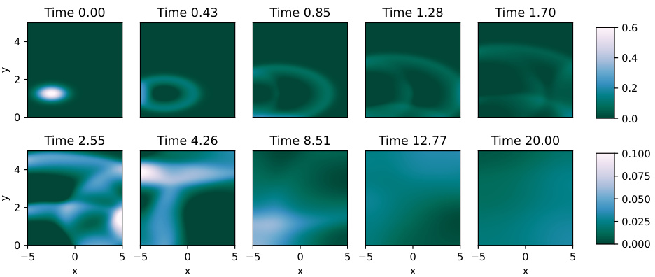
🔼 This figure shows the numerical solution of the shallow water equations (SWEs) at different time steps. The spatial domain is represented by x and y coordinates ranging from -5 to 5 and 0 to 5 respectively. The color scale represents the water depth (h), with blue indicating higher depths. The simulation starts with a Gaussian shaped water column and progresses to show the evolution over time as the water spreads out and interacts with the boundaries.
read the caption
Figure 2: Numerical solution of the SWE for (x, y) ∈ [−5,5] × [0,5] with Nx = 264 and Ny = 133 for a range of system times t. Only the water depth h (blue) is plotted.
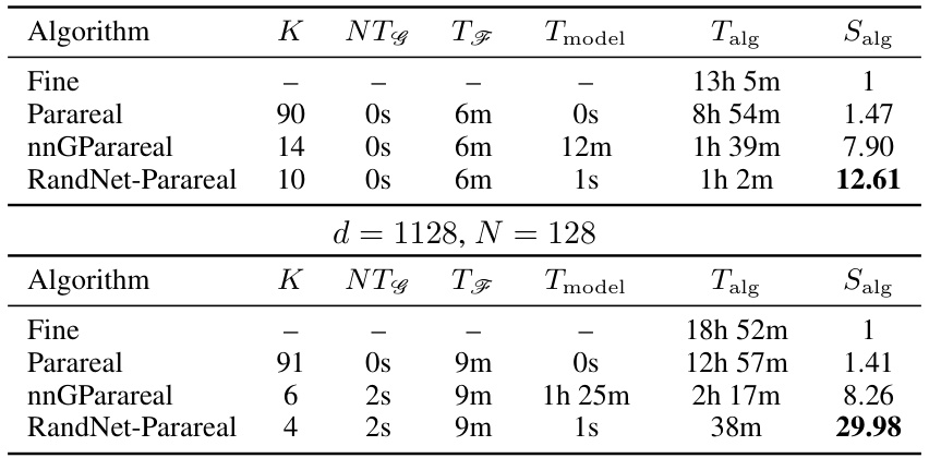
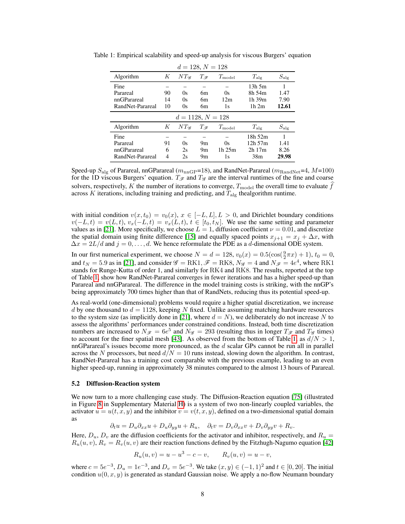
🔼 This table compares the performance of four different algorithms (Fine, Parareal, nnGParareal, and RandNet-Parareal) for solving the viscous Burgers’ equation. It shows the number of iterations (K) required for each algorithm to converge, the runtime of the coarse solver (NTG), the runtime of the fine solver (TF), the model training time (Tmodel), the total algorithm runtime (Talg), and the speedup (Salg) achieved compared to the fine solver run serially. Two different problem sizes (d = 128 and d = 1128) are considered, with N = 128 in both cases. The speedup (Salg) is calculated as the ratio of the serial runtime of the fine solver to the total runtime of the algorithm.
read the caption
Table 1: Empirical scalability and speed-up analysis for viscous Burgers' equation
In-depth insights#
RandNet-Parareal Intro#
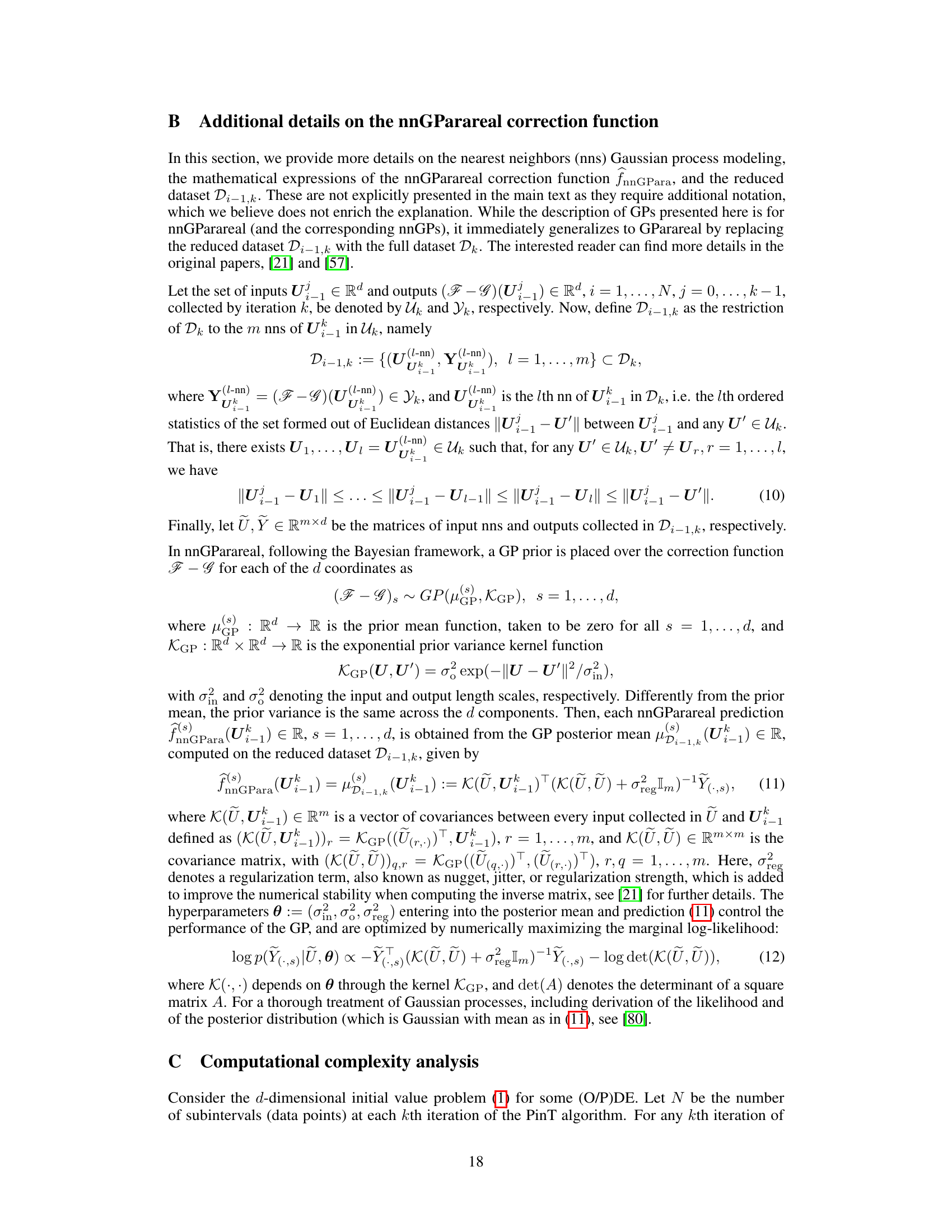
RandNet-Parareal, as a novel time-parallel PDE solver, presents a compelling blend of established numerical methods and cutting-edge machine learning techniques. The introduction would likely highlight the limitations of traditional spatial parallelism for solving computationally expensive initial value problems (IVPs) for ODEs and PDEs, motivating the need for parallel-in-time (PinT) methods like Parareal. RandNet-Parareal’s core innovation lies in its use of random neural networks (RandNets) to learn the discrepancy between a fast, approximate solver and an accurate, slow solver. This approach addresses the shortcomings of prior PinT methods, such as GParareal and nnGParareal, by avoiding computationally expensive Gaussian processes and significantly improving scalability. The introduction would set the stage by emphasizing RandNet-Parareal’s speed gains, potential for mesh scalability (handling up to 105 points), and applicability to a range of real-world problems. Theoretical guarantees concerning RandNets’ universal approximation capabilities would likely be mentioned, further bolstering the method’s reliability and robustness.
RandNet Architecture#
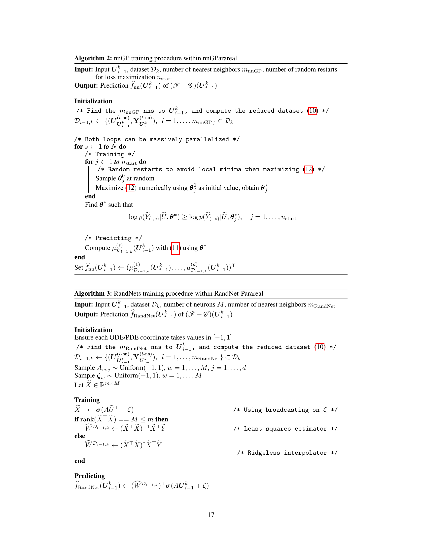
RandNet, a type of random neural network architecture, distinguishes itself through its randomly initialized and fixed hidden layer weights. Unlike traditional NNs that train all weights, RandNet only trains the output layer weights, significantly reducing training time and complexity. This simplification is achieved by randomly sampling the hidden layer’s parameters from a specified distribution and keeping them constant during the learning process. Consequently, the training boils down to solving a closed-form solution for the output weights through a least squares minimization, eliminating the need for backpropagation and addressing the vanishing/exploding gradient problems of deeper networks. This efficient training characteristic makes RandNet particularly attractive for applications such as learning discrepancies in the Parareal algorithm, as it allows for quick adaptation to new data and enhanced scalability, particularly when the number of dimensions is large.
Parallel Speed-up#
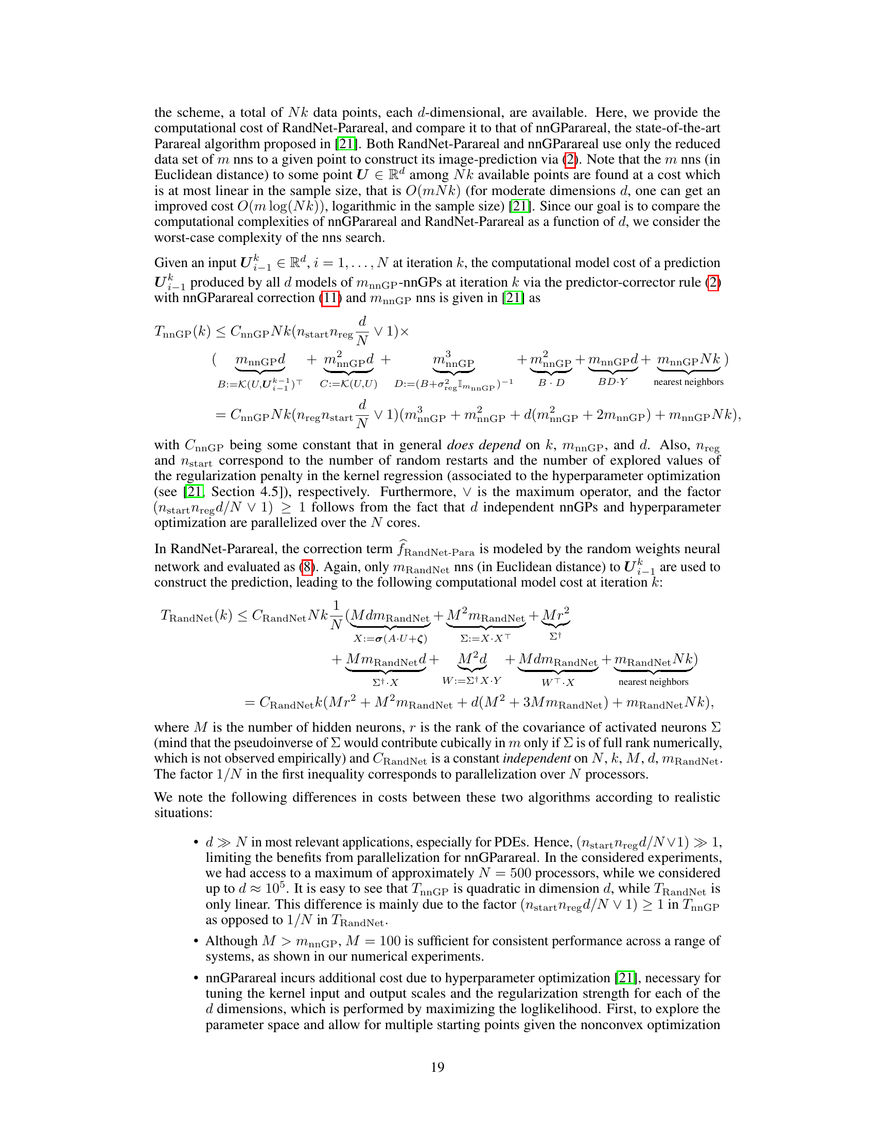
Analyzing parallel speed-up in this context necessitates a nuanced examination of the algorithm’s efficiency in leveraging parallel processing. RandNet-Parareal demonstrates significant speed improvements compared to traditional Parareal and its recent variant, nnGParareal. This enhancement stems from the algorithm’s effective use of random neural networks (RandNets) to learn the discrepancy between coarse and fine solutions, thus reducing computational cost. Speed gains of up to x125 compared to the serial fine solver, and x22 over standard Parareal, underscore the efficiency gains. However, the scalability and speed-up are heavily dependent on various factors, such as the dimensions of the problem and the number of processors. In scenarios with constrained resources or high dimensionality, the advantage of RandNet-Parareal becomes even more pronounced. Careful analysis of the training costs and iterative processes is crucial for a thorough understanding of its parallel speed-up capabilities.
Algorithm Robustness#
A robust algorithm maintains reliable performance across diverse conditions. Assessing algorithm robustness involves evaluating its sensitivity to variations in input data, parameters, and environmental factors. The primary goal is to determine the algorithm’s resilience to noise, outliers, and unexpected inputs, ensuring its continued effectiveness in real-world scenarios. This evaluation often involves rigorous testing with carefully designed experiments and statistical analysis. Key aspects to consider include the algorithm’s sensitivity to parameter changes, its ability to generalize to unseen data, and its resistance to adversarial attacks or malicious manipulations. A thorough robustness analysis is crucial for deploying algorithms reliably, especially in high-stakes applications.
Future Research#
Future research directions stemming from this RandNet-Parareal study could involve exploring alternative neural network architectures beyond RandNets to potentially enhance accuracy and efficiency further. Investigating the impact of different activation functions and weight initialization strategies would also be valuable. A comprehensive theoretical analysis to provide tighter error bounds and convergence rate guarantees for RandNet-Parareal, considering various problem settings, is needed. Furthermore, extending RandNet-Parareal to handle more complex PDEs, such as those with stochastic terms or non-linear boundary conditions, is a crucial next step. Finally, assessing the performance of RandNet-Parareal on diverse hardware architectures, including GPUs and specialized hardware accelerators, to maximize parallel efficiency and scalability is essential for broader adoption.
More visual insights#
More on figures

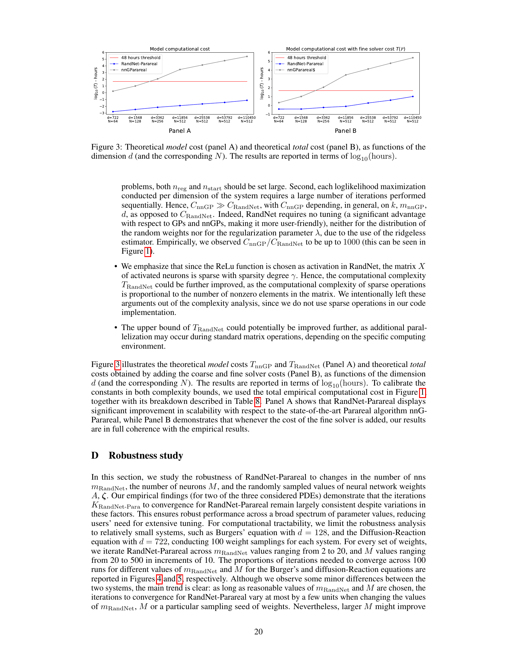
🔼 This figure displays a comparison of the computational costs of RandNet-Parareal and nnGParareal. Panel A shows the model computational cost, while Panel B includes the cost of the fine solver. The x-axis represents the dimension d (and the corresponding number of processors N), and the y-axis represents the log10 of the computational cost in hours. The figure shows that RandNet-Parareal has significantly lower computational costs than nnGParareal, especially for larger problem sizes.
read the caption
Figure 3: Theoretical model cost (panel A) and theoretical total cost (panel B), as functions of the dimension d (and the corresponding N). The results are reported in terms of log10(hours).

🔼 This figure shows the robustness of the RandNet-Parareal algorithm against variations in the number of nearest neighbors (mRandNet) and the number of neurons (M). For each of 100 different random weight initializations, the algorithm’s convergence rate (iterations to convergence) is evaluated across different values of mRandNet and M. The left panel displays the results for varying mRandNet, and the right panel displays the results for varying M. The stacked bars in each panel visually represent the distribution of convergence iterations across the tested parameter values.
read the caption
Figure 4: Histogram of the iterations to convergence KRandNet-Para of RandNet-Parareal for d = 128 for Burgers’ equation. We sample the network weights A, ζ 100 times. For each set of weights, we run RandNet-Parareal for mRandNet ∈ {2,3,..., 20} and M ∈ {20,30,40,...,500}. The left and right panels show the aggregated histograms of KRandNet-Para versus mRandNet and M, respectively.

🔼 This figure displays the robustness of RandNet-Parareal to the number of nearest neighbors (mRandNet) and the number of neurons (M) in the random neural network. The left panel shows the distribution of the number of iterations to convergence (KRandNet-Para) for different values of mRandNet, and the right panel shows this distribution for different values of M. The results suggest that RandNet-Parareal is relatively insensitive to variations in these hyperparameters.
read the caption
Figure 4: Histogram of the iterations to convergence KRandNet-Para of RandNet-Parareal for d = 128 for Burgers' equation. We sample the network weights A, ζ 100 times. For each set of weights, we run RandNet-Parareal for MRandNet ∈ {2,3,..., 20} and M ∈ {20,30,40,...,500}. The left and right panels show the aggregated histograms of KRandNet-Para versus MRandNet and M, respectively.

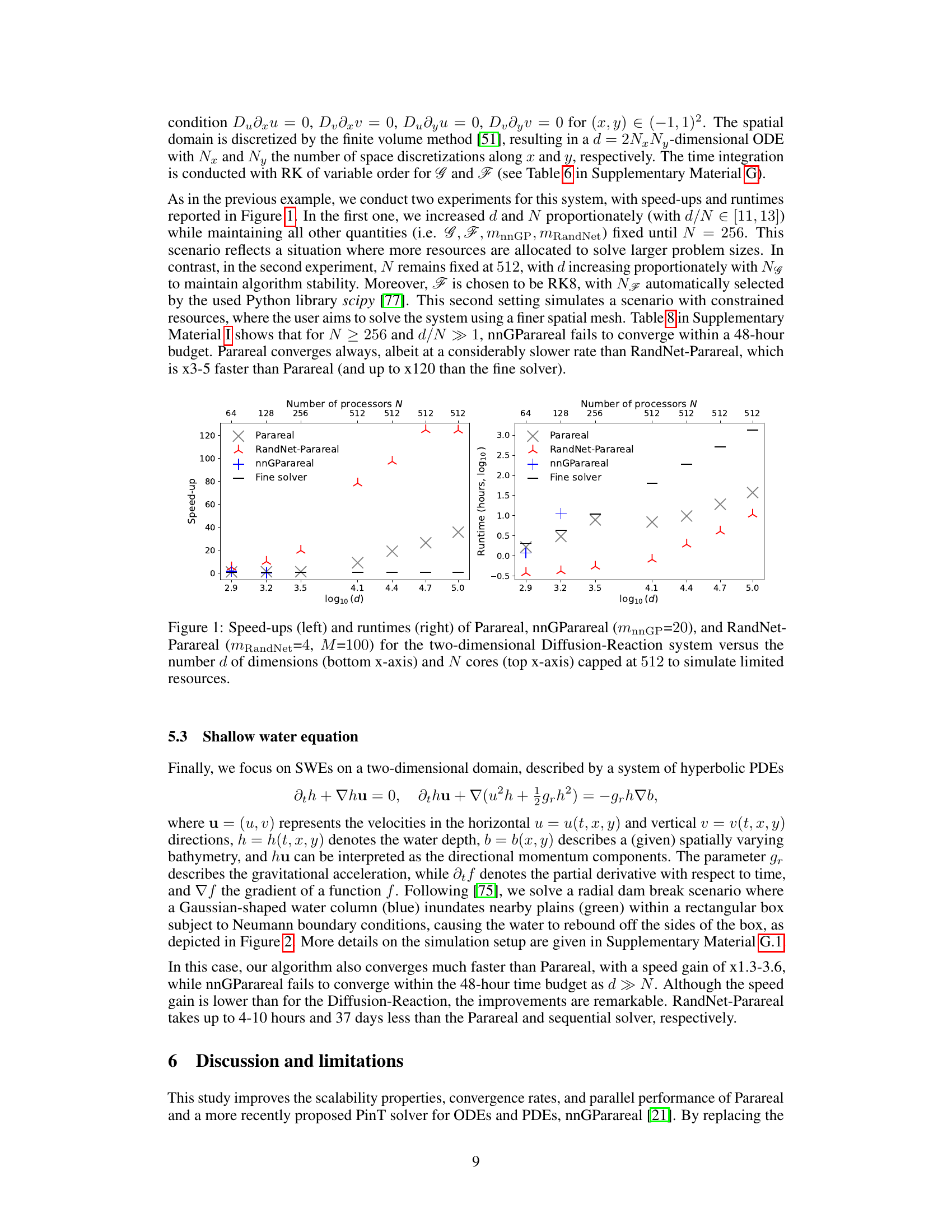
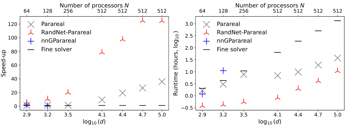
🔼 This figure compares the performance of three parallel-in-time (PinT) methods: Parareal, nnGParareal, and RandNet-Parareal for solving the two-dimensional Diffusion-Reaction system. The left panel shows the speedup achieved by each method, while the right panel shows the corresponding runtime. The x-axis represents the number of dimensions (d) and the number of cores (N), capped at 512 to simulate limited resources. The results demonstrate RandNet-Parareal’s significant performance improvement in terms of scalability and runtime.
read the caption
Figure 1: Speed-ups (left) and runtimes (right) of Parareal, nnGParareal (mnnGP=20), and RandNet-Parareal (MRandNet=4, M=100) for the two-dimensional Diffusion-Reaction system versus the number d of dimensions (bottom x-axis) and N cores (top x-axis) capped at 512 to simulate limited resources.

🔼 This figure shows the numerical solution of the viscous Burgers’ equation, a one-dimensional PDE exhibiting hyperbolic behavior, over the spatial domain [-1,1] and time interval [0,5.9]. The solution is obtained using a high spatial resolution with 1128 discretization points, representing a high-dimensional ODE system. The initial condition and other simulation parameters are detailed in Section 5.1 of the paper. The colormap represents the solution’s values across the spatial and temporal domains.
read the caption
Figure 7: Numerical solution of viscous Burgers' equation over (x,t) ∈ [-1,1] × [0,5.9] with d = 1128 and initial conditions and additional settings as described in Section 5.1.
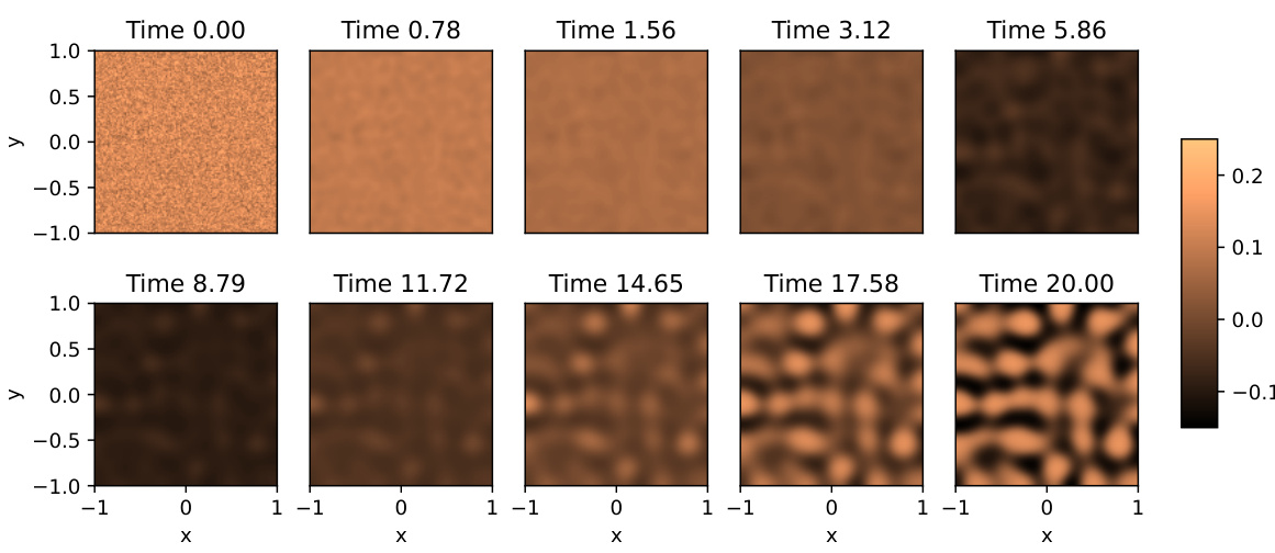
🔼 This figure shows the numerical solution of the Diffusion-Reaction equation at different time steps. The solution is displayed as a heatmap across a 2D spatial domain. It visualizes the activator u(t,x,y) concentration over time. The initial conditions and parameter settings are detailed in section 5.2 of the paper.
read the caption
Figure 8: Numerical solution of the Diffusion-Reaction equation over (x, y) ∈ [-1,1]² with Nx = Ny = 235 for a range of system times t. Only the activator u(t, x, y) is plotted. The initial conditions and additional settings are as described in Section 5.2.
More on tables
🔼 This table compares the performance of four different algorithms (Fine, Parareal, nnGParareal, and RandNet-Parareal) for solving the viscous Burgers’ equation. It shows the number of iterations (K) required for convergence, the runtimes of the coarse (TG) and fine (TF) solvers, the model training time (Tmodel), the total algorithm runtime (Talg), and the speedup (Salg) achieved by each algorithm. Two different problem sizes (d = 128 and d = 1128) are considered, demonstrating the scalability of each method.
read the caption
Table 1: Empirical scalability and speed-up analysis for viscous Burgers' equation

🔼 The table presents a speed-up analysis for solving the shallow water PDE using three different parallel-in-time algorithms: Parareal, RandNet-Parareal, and nnGParareal. The analysis considers varying spatial dimensions (d) of the system. For each dimension, it shows the number of iterations to convergence (K) for each algorithm, the runtime of the fine solver (Tg), the runtime of Parareal (Tpara), the runtime of RandNet-Parareal (TrandNet-Para), the speed-up of Parareal relative to the fine solver (SPara), and the speed-up of RandNet-Parareal relative to the fine solver (SRandNet-Para). The number of processors (N) is fixed at 235 for all experiments. This allows comparison of the scalability and performance of each algorithm in solving progressively larger PDE systems. nnGParareal fails to converge within the given time budget for the higher dimensional problems.
read the caption
Table 2: Speed-up analysis for the shallow water PDE as a d-dimensional ODE system, N = 235

🔼 This table details the simulation parameters used for the 2D and 3D Brusselator experiments. It specifies the spatial domain, the number of discretization points for u and v (Nu and Nv), the resulting dimensionality (d) of the ODE system, the coarse and fine solvers used (G and F), their respective time steps (GΔt and FΔt), and the number of intervals (N). The table helps clarify the computational setup and parameters used in the experiments comparing RandNet-Parareal’s performance against Parareal and nnGParareal.
read the caption
Table 3: Simulation setup for the 2D and 3D Brusselator

🔼 This table compares the accuracy and computational cost (runtime) of RandNet-Parareal, Parareal, and nnGParareal across six different partial differential equation (PDE) systems. Accuracy is measured as the maximum absolute error (mean across intervals) compared to the true solution from a sequential run of the fine solver. The table shows that RandNet-Parareal achieves significantly better accuracy and lower runtimes compared to the other two methods, especially for larger-scale problems where nnGParareal fails to converge.
read the caption
Table 4: Accuracy and computational cost of the three considered algorithms

🔼 This table presents a comparison of the performance of three algorithms (Fine, Parareal, nnGParareal, and RandNet-Parareal) for solving the viscous Burgers’ equation. The comparison is done for two different spatial dimensions (d = 128 and d = 1128) keeping the number of intervals fixed at N=128. For each algorithm and dimension, the table shows the number of iterations (K) required for convergence, the runtime of the fine solver (TF), runtime of the coarse solver (TG), model training time (Tmodel), total algorithm runtime (Talg), and speedup (Salg) relative to the serial runtime of the fine solver. The speedup highlights the performance gains achieved by the parallel-in-time methods compared to solving the problem sequentially using the fine solver. The model training times emphasize the computational cost difference in building the correction function among the algorithms.
read the caption
Table 1: Empirical scalability and speed-up analysis for viscous Burgers' equation

🔼 This table details the simulation setup used for the Diffusion-Reaction equation experiments. It specifies the spatial domain, the number of spatial discretization points along each axis (Nx and Ny), the resulting dimensionality of the ODE system (d), the coarse and fine solvers (G and F), the number of timesteps per interval (Ng and NF), and the total number of intervals (N). The specific solvers used are Runge-Kutta methods of order 1 (RK1), 4 (RK4), and 8 (RK8). The number of nearest neighbors (nnGP and RandNet-Parareal) used in nnGParareal and RandNet-Parareal are not explicitly included but are mentioned in the text.
read the caption
Table 6: Simulation setup for the Diffusion-Reaction equation

🔼 This table details the simulation setup for the Shallow Water Equations (SWEs) experiments. It shows the spatial domain, the number of spatial discretization points in the x and y directions (Nx and Ny), resulting in a total of d dimensions for the ordinary differential equation (ODE) system that represents the SWE. The table also specifies the coarse and fine numerical solvers (G and F), the corresponding number of time steps per interval (Ng and NF), and the total number of intervals (N) used in the simulations. The number of nearest neighbors used for nnGParareal and RandNet-Parareal are also provided (mnnGP and mRandNet).
read the caption
Table 7: Simulation setup for the SWEs
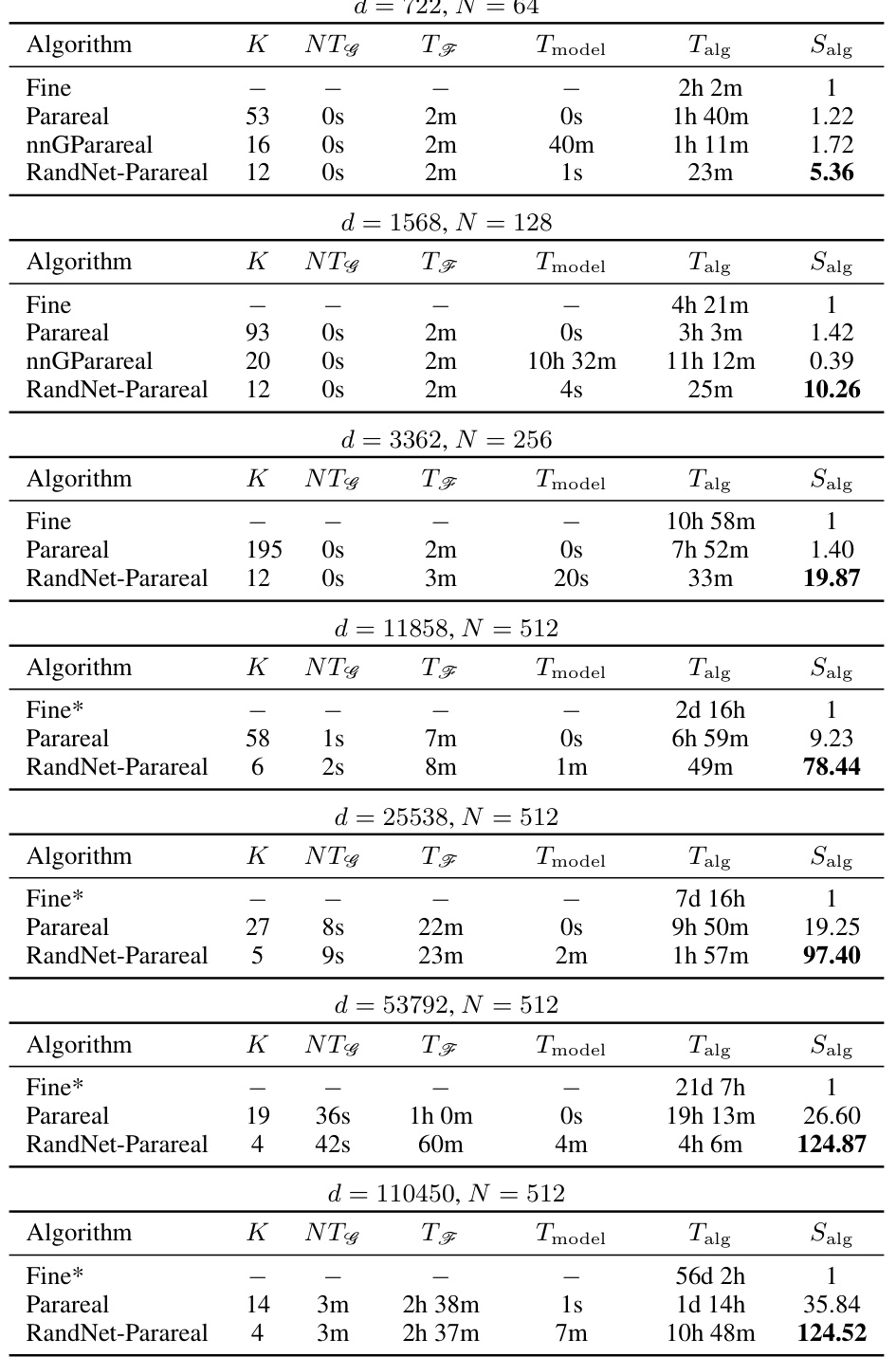
🔼 This table presents a comparison of the performance of three parallel-in-time (PinT) algorithms: Parareal, nnGParareal, and RandNet-Parareal, on the one-dimensional viscous Burgers’ equation. The table shows the number of iterations (K) required for convergence, the runtimes of the coarse and fine solvers (NTG, TF), the model training time (Tmodel), the total algorithm runtime (Talg), and the speed-up achieved compared to the serial runtime of the fine solver (Salg). The table includes results for two different problem sizes: d = 128 and d = 1128, demonstrating the scalability of the algorithms as the problem size increases.
read the caption
Table 1: Empirical scalability and speed-up analysis for viscous Burgers' equation
Full paper#


