TL;DR#
Solving constrained nonlinear programs (NLPs) is computationally expensive, especially for large-scale problems frequently encountered in power systems, robotics, and wireless networks. The interior point method (IPM) is a popular approach for solving NLPs; however, its performance is hampered by the need to solve large systems of linear equations. This paper addresses this computational bottleneck by proposing IPM-LSTM.
IPM-LSTM uses LSTM neural networks to efficiently approximate solutions to these linear systems, significantly reducing the computational burden of the IPM. The approximated solutions are then used to warm-start a standard interior point solver, which further enhances the speed and efficiency of NLP solving. The results demonstrate that IPM-LSTM outperforms traditional methods, achieving substantial improvements in solution time and iteration count across various NLP types, including quadratic programs and quadratically constrained quadratic programs.
Key Takeaways#
Why does it matter?#
This paper is crucial because it presents a novel approach to accelerate nonlinear program (NLP) solving, a computationally expensive task prevalent in many fields. By integrating LSTM networks into the interior point method, it offers a significant speedup with potential applications across diverse domains. This opens new avenues for research on learning-based optimization techniques and their integration with classic methods. The results are promising and encourage further investigations into the synergy of machine learning and optimization.
Visual Insights#

🔼 This figure illustrates the IPM-LSTM approach, which integrates Long Short-Term Memory (LSTM) neural networks into an interior point method (IPM) to accelerate solving nonlinear programs (NLPs). The IPM-LSTM approach uses LSTM networks to approximate solutions to the systems of linear equations that are computationally expensive within the standard IPM. These approximate solutions then warm-start a standard interior point solver (like IPOPT) to further refine the solution and obtain the optimal solution. The figure shows the LSTM networks approximating the solution of the linear system, and how that approximate solution is passed to the IPOPT solver as a warm start.
read the caption
Figure 1: An illustration of the IPM-LSTM approach.
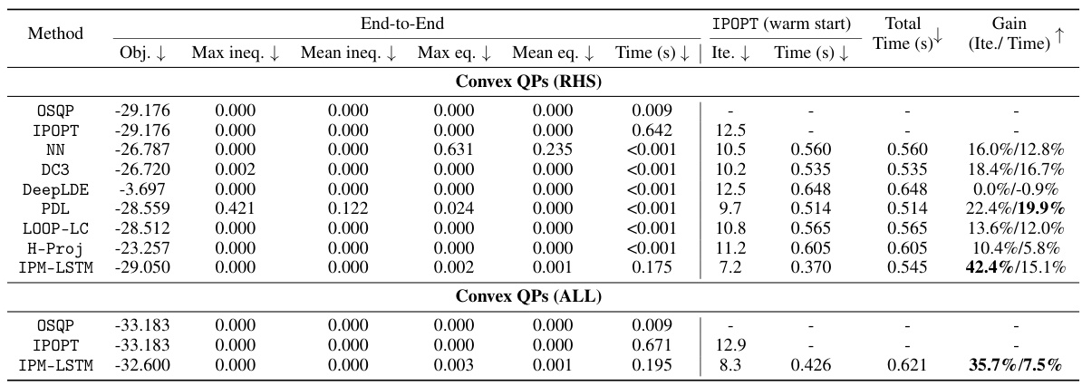
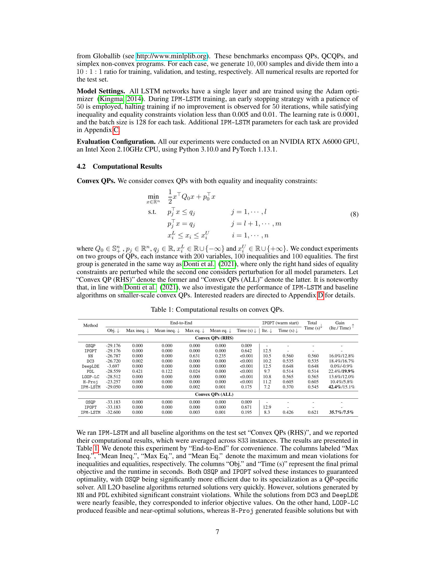
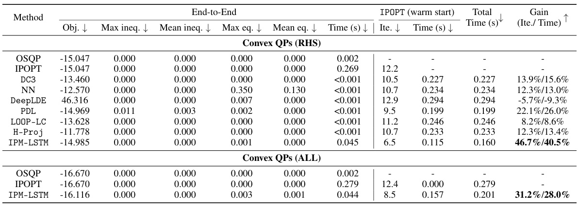
🔼 This table presents the computational results of various optimization algorithms on two sets of convex quadratic programs (QPs). The first set, ‘Convex QPs (RHS)’, involves perturbing only the right-hand sides of the equality constraints, while the second set, ‘Convex QPs (ALL)’, perturbs all model parameters. The table compares the performance of OSQP, IPOPT, and several learning-to-optimize (L2O) approaches, including NN, DC3, DeepLDE, PDL, LOOP-LC, and H-Proj, against the proposed IPM-LSTM method. For each algorithm, it reports the objective value, constraint violations (maximum and mean for inequalities and equalities), solution time, number of iterations, and the percentage gain in iterations and solution time compared to the default IPOPT solver when using the algorithm’s solution as a warm start for IPOPT. This allows for a comprehensive comparison of the effectiveness and efficiency of different optimization methods in solving convex QPs under varying perturbation scenarios.
read the caption
Table 1: Computational results on convex QPs.
In-depth insights#
IPM-LSTM Approach#
The IPM-LSTM approach presents a novel method for solving nonlinear programs (NLPs) by integrating a Long Short-Term Memory (LSTM) neural network into the classic interior point method (IPM). The core innovation lies in using the LSTM to approximate solutions to the linear systems that arise in each IPM iteration. This approximation significantly reduces the computational cost associated with matrix factorization, a major bottleneck in traditional IPMs. The LSTM is trained in a self-supervised manner, learning to predict near-optimal solutions for the linear systems, effectively leveraging the power of deep learning to accelerate a classical optimization algorithm. The approximated solution obtained is then used to warm-start a conventional interior point solver like IPOPT, further enhancing efficiency. This two-stage framework combines the strengths of both learning-based optimization and established IPM techniques. The results demonstrate a substantial improvement, showcasing significant reductions in both the number of iterations and overall solution time compared to using the default solver alone. The method’s applicability to various NLP types, including quadratic programs (QPs) and quadratically constrained quadratic programs (QCQPs), highlights its potential as a general-purpose acceleration technique for NLP solvers.
LSTM Network#
In the context of a research paper, a section on “LSTM Networks” would delve into the specifics of employing Long Short-Term Memory networks. It would likely begin by establishing the rationale for choosing LSTMs over other recurrent neural network architectures, highlighting LSTMs’ unique ability to handle long-range dependencies in sequential data, a crucial feature when processing time-series information. The discussion would then elaborate on the network architecture, detailing the cell structure comprising input, forget, cell, and output gates. The training process, using techniques like backpropagation through time (BPTT), is also key. A critical aspect would be the loss function selection and optimization algorithms used to adjust the network’s weights to minimize error. Further, the section should discuss hyperparameter tuning (number of layers, neurons per layer, etc.), along with validation strategies to avoid overfitting. Finally, it’s important to analyze the computational complexity and potential limitations of LSTMs, such as vanishing/exploding gradients and the difficulty in interpreting their internal representations. Overall, a comprehensive “LSTM Network” section would showcase a deep understanding of LSTM architecture and its practical implementation in the specific context of the paper.
NLP Solution#
A hypothetical NLP solution section in a research paper would delve into the specific techniques employed to address a natural language processing problem. It would likely detail the chosen model architecture, for example, a transformer network, along with crucial design choices such as layer depth, attention mechanisms, and any specialized modifications. Data preprocessing steps are paramount, outlining the cleaning, tokenization, and potentially feature engineering implemented. The section would meticulously explain the training process, including the objective function, optimization algorithm used (e.g., AdamW), and hyperparameter tuning strategies. Evaluation metrics are crucial, showcasing how the model’s performance was assessed (e.g., accuracy, F1-score, BLEU). Crucially, the NLP solution would analyze and interpret the results, comparing them to baseline models and discussing strengths, weaknesses, and areas for future improvement. Addressing limitations and potential biases inherent in the dataset or methodology is also essential for a robust NLP solution.
Two-Stage Model#
A two-stage model is a powerful approach to solving complex problems by breaking them into two more manageable parts. The first stage often involves a preliminary step such as feature extraction, model training, or creating an initial guess. This initial result is then used to inform and improve a more refined second stage. The second stage builds upon the first, leveraging the results to increase efficiency or accuracy. This approach can lead to a significant improvement over a single-stage approach. This method is particularly useful when the computational cost of the second stage is high. By using the first stage as a warm-start, the second stage requires fewer iterations, thereby significantly reducing solution time. Moreover, the two-stage method can lead to superior performance regarding both feasibility and optimality by creating a more robust and efficient process. Error handling and robustness are enhanced as issues are identified and addressed in the first stage before proceeding to the computationally expensive second stage.
Future Works#
Future work could explore several promising directions. Extending IPM-LSTM to handle a broader range of NLP problem types is crucial, including non-convex problems with complex constraints or those involving large-scale datasets. Investigating alternative neural network architectures beyond LSTMs, such as transformers or graph neural networks, could potentially improve approximation accuracy and efficiency. Improving the robustness of the IPM-LSTM approach against noisy or incomplete data is another critical area. This could involve developing more sophisticated regularization techniques or incorporating uncertainty estimation methods. Combining IPM-LSTM with other optimization techniques, such as proximal methods or augmented Lagrangian methods, may lead to further improvements. Finally, thorough theoretical analysis of the convergence properties and computational complexity of IPM-LSTM is needed to solidify its foundation and guide future development. A detailed empirical comparison with state-of-the-art L2O techniques on a wider range of benchmarks would also enhance the paper’s impact.
More visual insights#
More on figures

🔼 This figure illustrates the LSTM network architecture used for approximating solutions to the linear systems within the IPM. The architecture consists of multiple LSTM cells, each taking as input the previous estimate (yt-1) and the gradient of the loss function (∇Φ(yt-1)). The LSTM cell processes these inputs using its internal mechanisms (gates and activation functions) to produce a new estimate (yt). This process is repeated across T LSTM cells, resulting in a final approximate solution yT to the least squares problem. The figure also highlights the sharing of parameters across different LSTM cells and coordinates of y, which improves efficiency and generalizability.
read the caption
Figure 2: The LSTM architecture for solving min Φ(y).

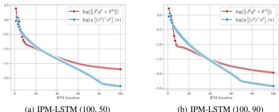
🔼 This figure shows the performance analysis of IPM-LSTM on a convex QP (RHS) problem. The four subfigures illustrate (a) Condition (5): the relation between the norm of Jkyk + Fk and η[(zk)Txk]/n; (b) Condition (6): the relation between ||yk|| and (1+σ+η)||Fo(xk,λk,zk)||; (c) Residual: the value of ||Jkyk + Fk|| across different LSTM time steps; (d) Objective value: the objective value across IPM iterations. The plots show that IPM-LSTM satisfies Assumption 1 during most of the iterations and that the approximation quality of the solution to the linear systems improves with the number of LSTM time steps. Also, the objective value decreases monotonically toward the optimal value with the increasing number of iterations.
read the caption
Figure 3: The performance analysis of IPM-LSTM on a convex QP (RHS).
🔼 This figure presents four subplots that analyze the performance of the IPM-LSTM algorithm on a convex quadratic program (QP) with 100 variables, 50 inequality constraints, and 50 equality constraints. Plot (a) shows the progress of ||Jkyk + Fk|| (the residual of the linear system at each iteration k) compared to η[(zk)Txk]/n (a condition for convergence of the algorithm) during IPM iterations. Plot (b) shows the progress of ||yk|| (the norm of the approximate solution) versus a bound on it related to the optimality gap. Plot (c) shows how the residual of the linear system decreases as the number of LSTM time steps increases, illustrating that LSTM networks improve solution quality with more time steps. Finally, plot (d) illustrates the convergence of the IPM-LSTM algorithm, showing that the objective function value decreases monotonically and converges toward the optimal value.
read the caption
Figure 3: The performance analysis of IPM-LSTM on a convex QP (RHS).

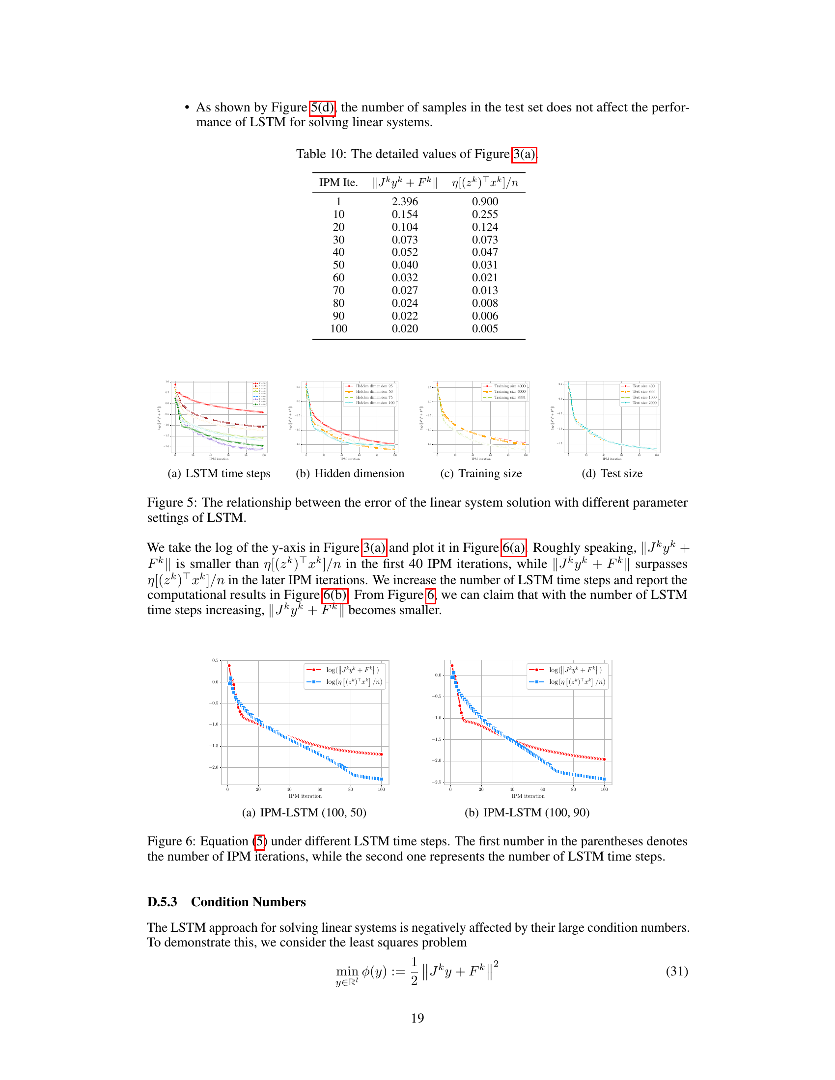
🔼 This figure illustrates the IPM-LSTM approach, showing how Long Short-Term Memory (LSTM) neural networks are integrated into an interior point method (IPM) to approximate solutions to linear systems. The approximated solutions are then used to warm-start an interior point solver (IPOPT), leading to a more efficient solution of the nonlinear program (NLP). The figure shows the LSTM cells approximating the solution to the linear system, which is then passed to the IPOPT solver as a warm start. The IPM-LSTM approach combines machine learning techniques with a classic optimization algorithm for improved performance.
read the caption
Figure 1: An illustration of the IPM-LSTM approach.
🔼 This figure illustrates the IPM-LSTM approach, showing how an LSTM neural network approximates solutions to linear systems within an Interior Point Method (IPM). The LSTM’s output is then used to warm-start the IPOPT solver, accelerating the overall NLP solving process. The diagram shows the IPM-LSTM architecture, highlighting the integration of LSTM cells into the main IPM algorithm to approximate solutions and improve efficiency.
read the caption
Figure 1: An illustration of the IPM-LSTM approach.
More on tables

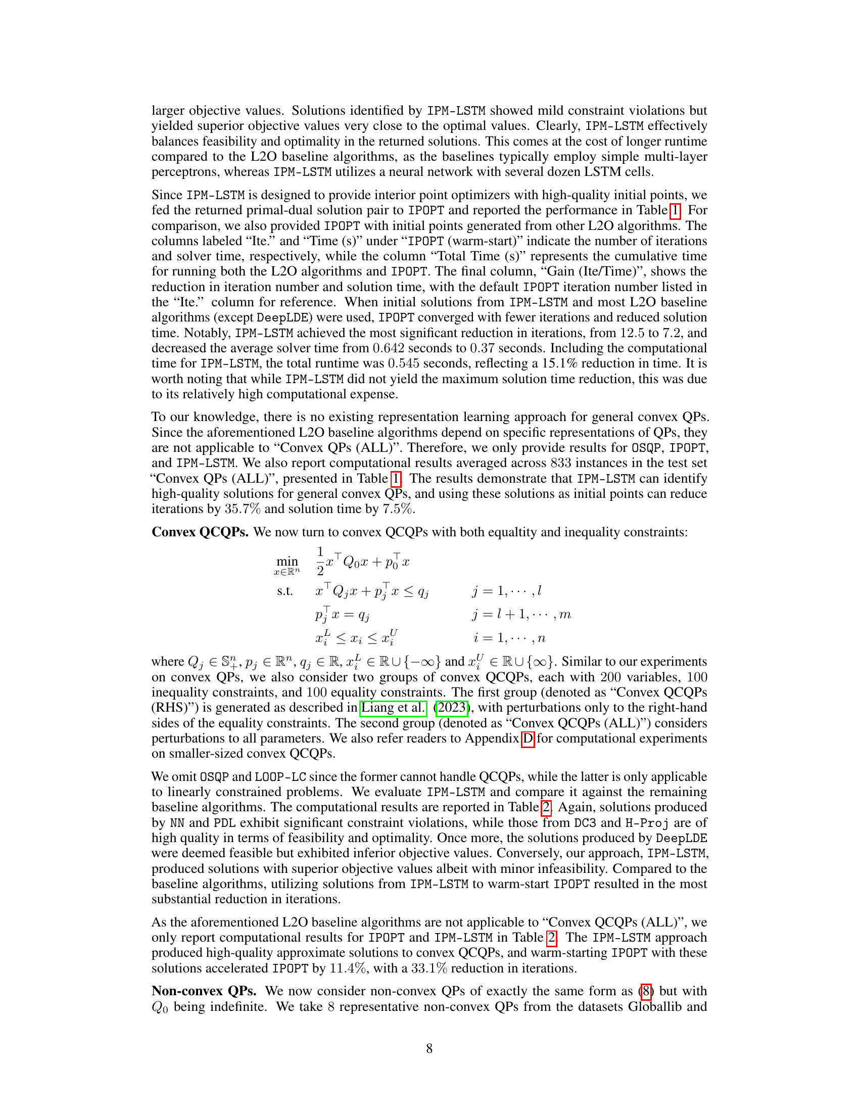
🔼 This table presents the computational results of various algorithms on convex QCQPs. It compares the performance of IPM-LSTM against traditional optimizers (IPOPT) and other learning-based optimization approaches (NN, DC3, DeepLDE, PDL, LOOP-LC, H-Proj). The table shows objective function values, constraint violations (maximum and mean for inequalities and equalities), and solution times. Separate results are given for two experimental settings: Convex QCQPs (RHS), where only the right-hand sides of equality constraints are perturbed, and Convex QCQPs (ALL), where all model parameters are perturbed. For IPM-LSTM, it also includes the results obtained after using its output as a warm start for IPOPT. The ‘Gain’ column shows the percentage improvement in iterations and time achieved using IPM-LSTM compared to the default IPOPT solver.
read the caption
Table 2: Computational results on convex QCQPs.

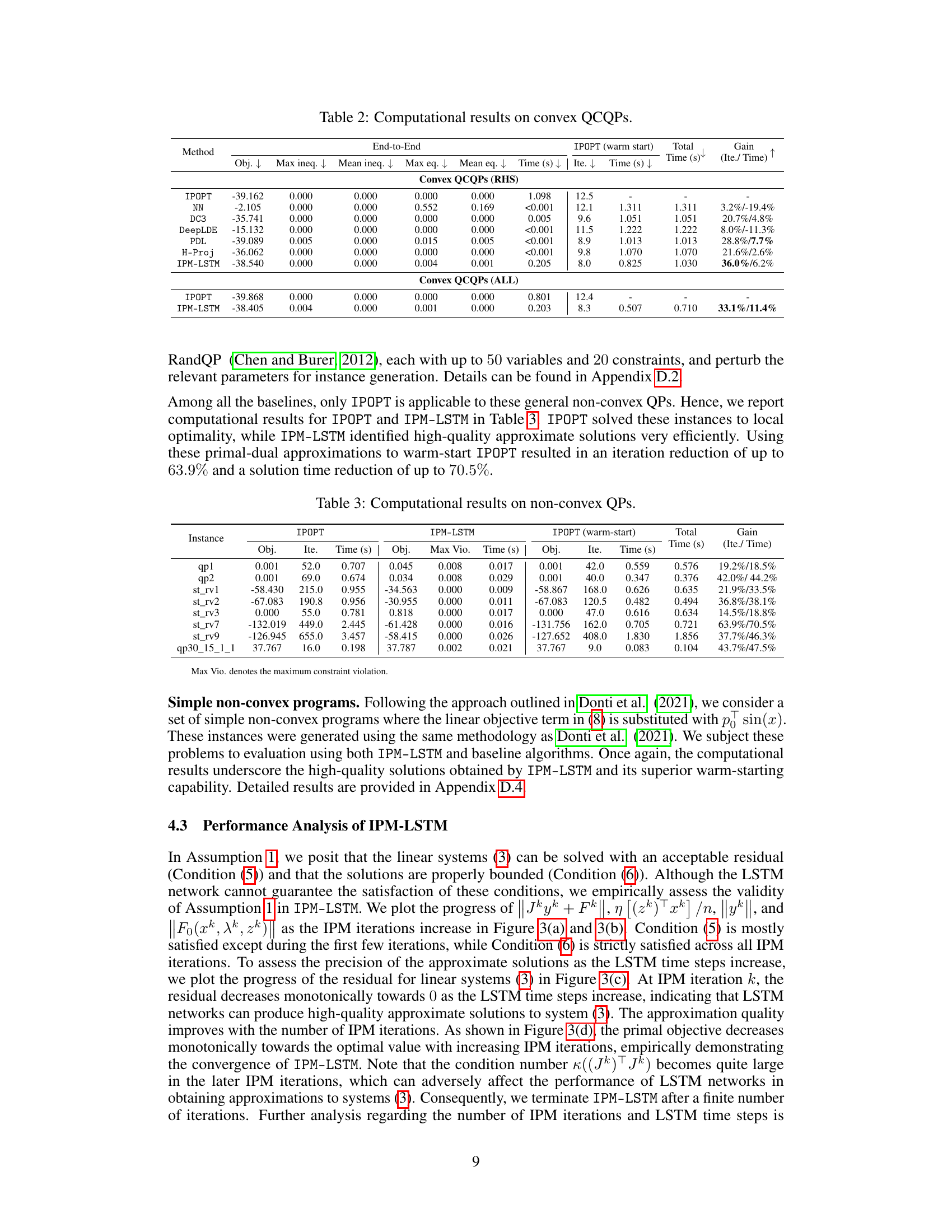
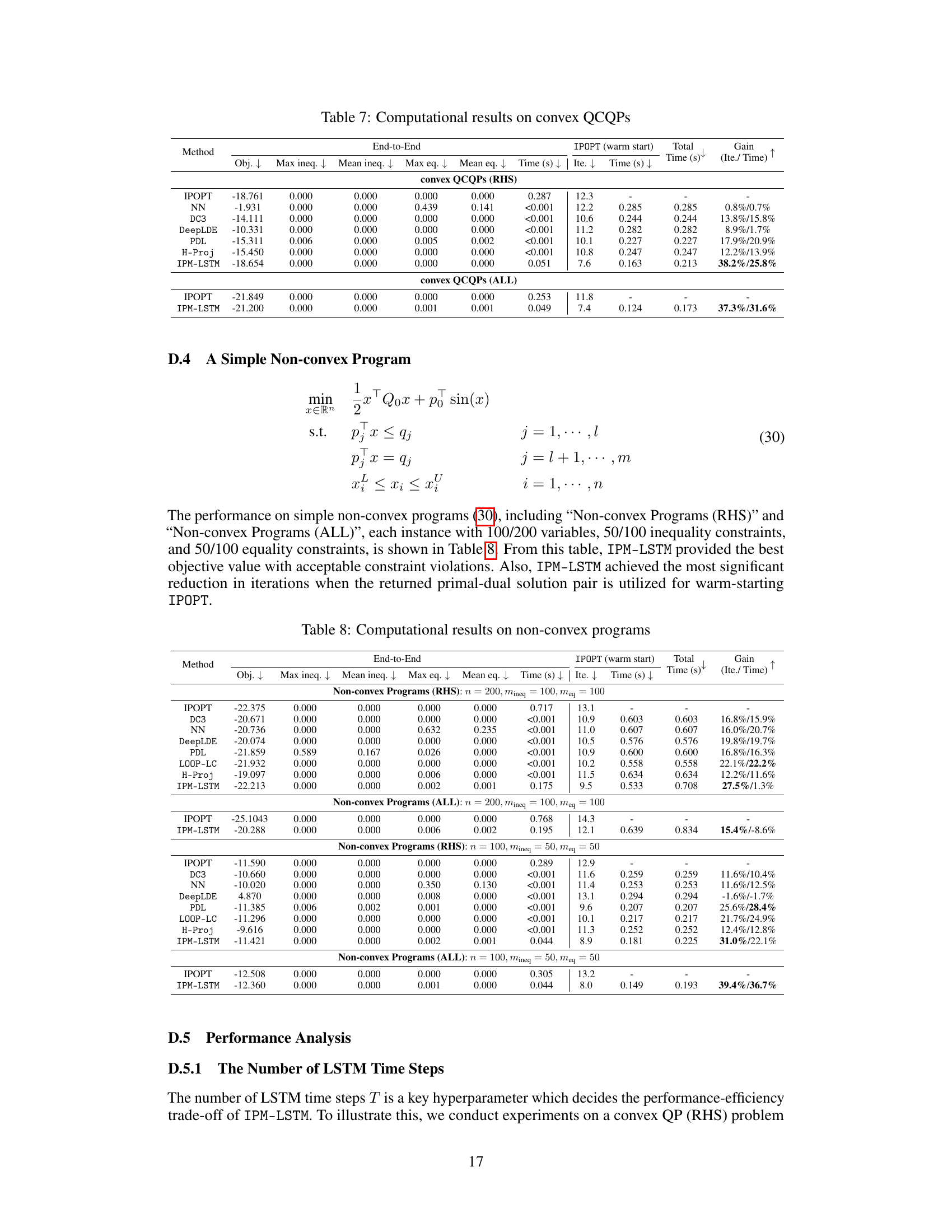
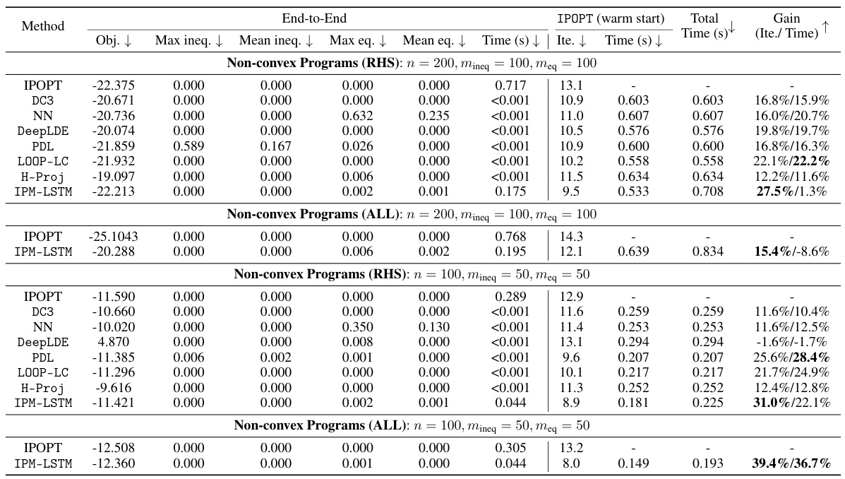
🔼 This table presents the computational results for non-convex quadratic programs (QPs). It compares the performance of IPOPT (a state-of-the-art interior point method) alone against IPM-LSTM followed by IPOPT (warm-start). The table shows the objective function value (Obj.), the number of iterations (Ite.), and the solution time (Time (s)) for each solver. The ‘Max Vio.’ column indicates the maximum constraint violation observed for IPM-LSTM. The ‘Total Time (s)’ column represents the total time taken by the IPM-LSTM and IPOPT (warm-start) pipeline. Finally, the ‘Gain (Ite./ Time)’ column shows the percentage improvement in the number of iterations and solution time achieved by using IPM-LSTM to warm-start IPOPT, compared to using IPOPT alone.
read the caption
Table 3: Computational results on non-convex QPs.

🔼 This table presents the computational results for various algorithms on convex quadratic programming problems. It compares the performance of IPM-LSTM against baseline algorithms (OSQP, IPOPT, NN, DC3, DeepLDE, PDL, LOOP-LC, H-Proj) across two sets of convex QPs (‘Convex QPs (RHS)’ and ‘Convex QPs (ALL)’). The results include the objective function value, maximum and mean constraint violations, solution time, and number of iterations. The table also shows the gain achieved by using IPM-LSTM’s approximate solution to warm-start the IPOPT solver, highlighting improvements in both iterations and solution time.
read the caption
Table 1: Computational results on convex QPs.
🔼 This table presents the computational results of various optimization algorithms on two sets of convex Quadratic Programs (QPs). The first set, ‘Convex QPs (RHS)’, involves perturbing only the right-hand sides of equality constraints, while the second set, ‘Convex QPs (ALL)’, perturbs all model parameters. The table compares the performance of OSQP, IPOPT, NN, DC3, DeepLDE, PDL, LOOP-LC, H-Proj, and IPM-LSTM in terms of objective function value, constraint violations, solution time, and the number of iterations. It also shows the improvements achieved when using the approximate solutions from IPM-LSTM to warm-start IPOPT.
read the caption
Table 1: Computational results on convex QPs.

🔼 This table describes the perturbation rules applied to the parameters of the non-convex quadratic programming problems used in the experiments. For each problem instance (listed in the first column), the table shows whether each parameter type (Qo, po, pineq, qineq, peq, qeq, xL, xU) underwent perturbation using either the ‘p’ (multiply by a random value between 0.8 and 1.2 and round if original is an integer), ‘r’ (round to the nearest integer), or ‘c’ (no perturbation) methods. This indicates how the input data was modified to create the problem instances for the evaluation of IPM-LSTM and other algorithms.
read the caption
Table 6: Perturbation rules.

🔼 This table presents the computational results of various methods (OSQP, IPOPT, NN, DC3, DeepLDE, PDL, LOOP-LC, H-Proj, and IPM-LSTM) for solving convex quadratic programs (QPs). The results are divided into two groups: Convex QPs (RHS), where only the right-hand sides of the equality constraints are perturbed, and Convex QPs (ALL), where all model parameters are perturbed. For each method, the table shows the objective function value, maximum and mean constraint violations (inequality and equality), and the solution time and number of iterations. It also shows the speedup achieved by warm-starting IPOPT with solutions generated by each method. The results highlight the performance improvements achieved by IPM-LSTM, particularly when used to warm-start IPOPT.
read the caption
Table 1: Computational results on convex QPs.
🔼 This table presents a comparison of computational results for solving convex quadratic programming problems (QPs) using various methods. The methods compared include IPM-LSTM (the proposed method), OSQP, IPOPT, NN, DC3, DeepLDE, PDL, LOOP-LC, and H-Proj. The table shows the objective function value achieved by each method, maximum and mean constraint violations (inequality and equality constraints), the computation time, and the number of iterations. The results are further categorized by problem type (RHS and ALL) and show the improvements achieved using IPM-LSTM, including warm starts with IPOPT, in terms of solution time and the number of iterations.
read the caption
Table 1: Computational results on convex QPs.

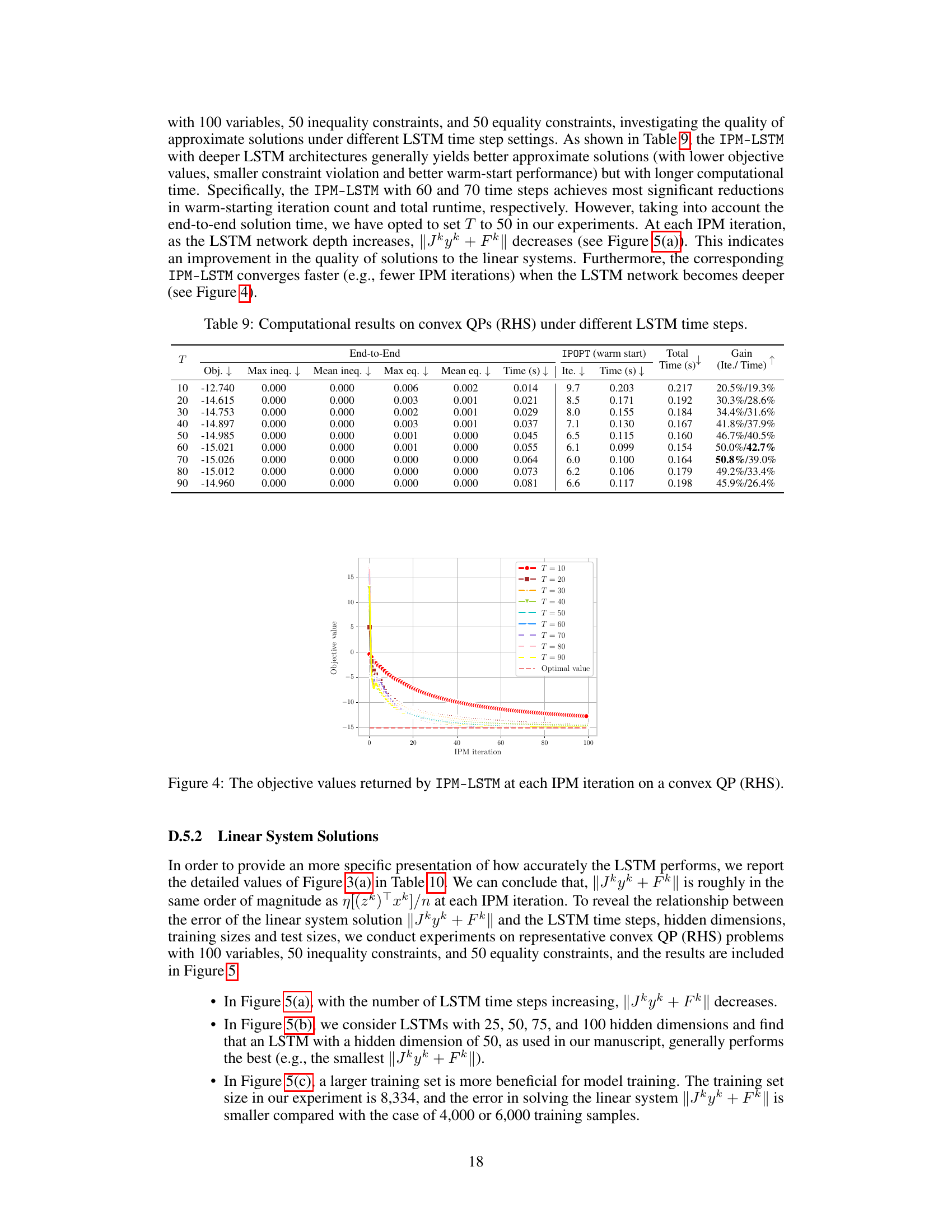
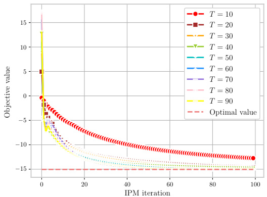
🔼 This table presents the computational results of the IPM-LSTM algorithm on convex quadratic programs with different numbers of LSTM time steps (T). It compares the objective function values, constraint violations (maximum and mean for both inequality and equality constraints), solution times, and the number of iterations for both the end-to-end IPM-LSTM and when using IPM-LSTM to warm-start IPOPT. The ‘Gain’ column shows the percentage improvement in iterations and time achieved by using the warm-start approach compared to using IPOPT alone.
read the caption
Table 9: Computational results on convex QPs (RHS) under different LSTM time steps.
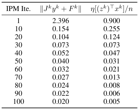
🔼 This table provides the numerical data corresponding to the plot in Figure 3(a) of the paper. It shows the values of ||Jkyk + Fk|| and η[(zk)Txk]/n at each IPM iteration. These values are important for assessing the accuracy and convergence of the IPM-LSTM algorithm, specifically relating to Assumption 1, which bounds the error of the approximate solution to the linear system at each iteration.
read the caption
Table 10: The detailed values of Figure 3(a).

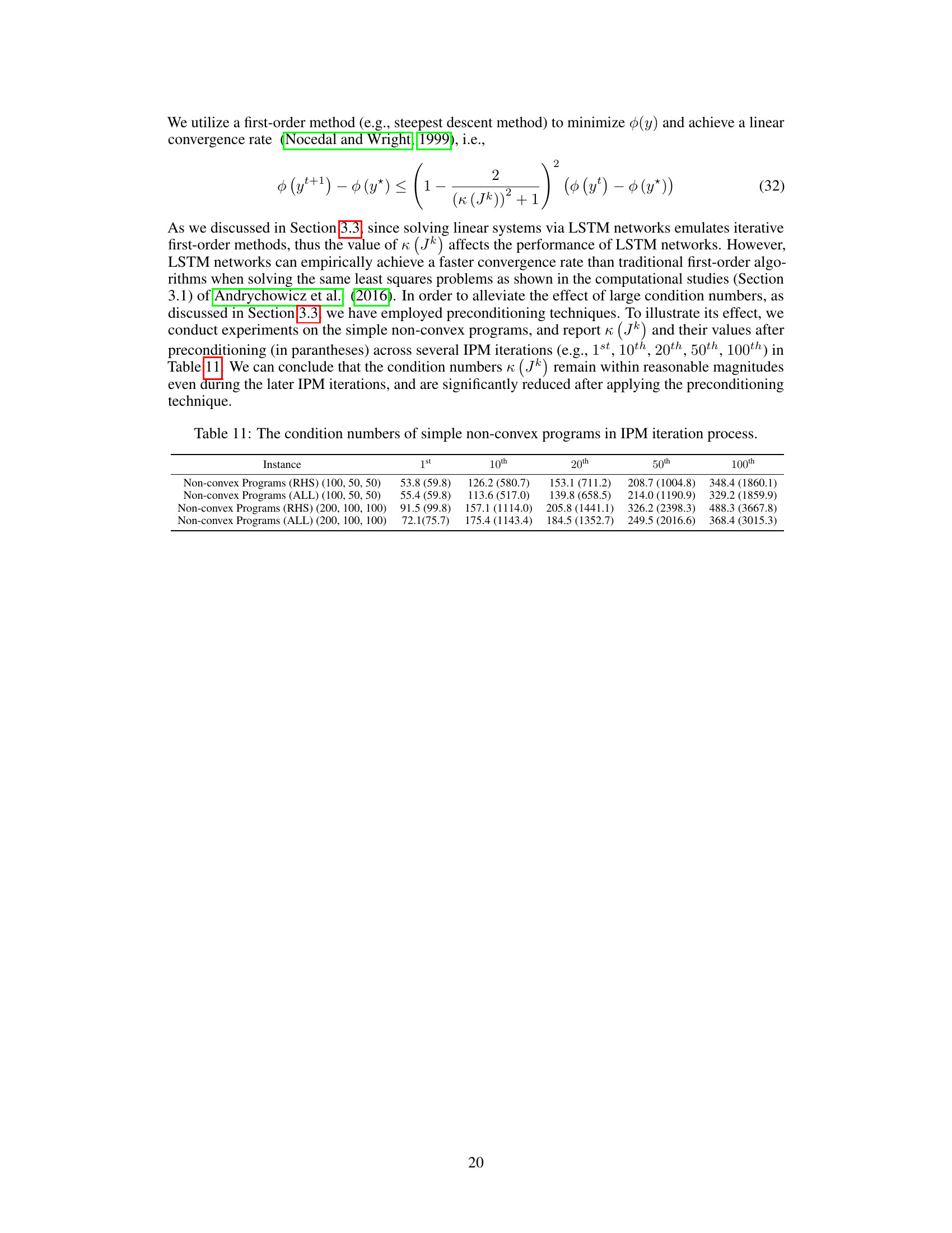
🔼 This table presents the condition numbers (κ(Jk)) of the Jacobian matrices (Jk) involved in solving linear systems within the IPM algorithm for different non-convex program instances across several IPM iterations (1st, 10th, 20th, 50th, 100th). The values in parentheses represent the condition numbers after applying a preconditioning technique. The table highlights how the condition numbers evolve during the iterative process and demonstrates the effect of preconditioning in maintaining reasonable magnitudes of these numbers, even in later iterations.
read the caption
Table 11: The condition numbers of simple non-convex programs in IPM iteration process.
Full paper#


