TL;DR#
Subgraph GNNs significantly enhance the expressive power of standard GNNs but suffer from scalability issues due to the large number of subgraphs processed. Previous attempts to improve scalability through subgraph sampling have proven suboptimal, yielding either poor performance or limitations on subset sizes. This substantially restricts their applicability to large-scale graph datasets, a crucial limitation for practical implementation.
This research introduces a novel Subgraph GNN framework that addresses this limitation. By associating subgraphs with node clusters rather than individual nodes and utilizing graph products and a coarsening function, this method achieves flexible subgraph selection, thereby improving scalability. It further enhances performance by identifying and utilizing novel permutation symmetries within node feature tensors. This approach is demonstrably more flexible and consistently outperforms baseline methods across multiple graph learning benchmarks.
Key Takeaways#
Why does it matter?#
This paper is crucial for researchers working on Subgraph Graph Neural Networks (GNNs). It offers a flexible and scalable framework that significantly improves upon existing methods, opening doors for more efficient and expressive GNN models that can handle large datasets. This is particularly important given the growing need for scalable GNNs in real-world applications.
Visual Insights#

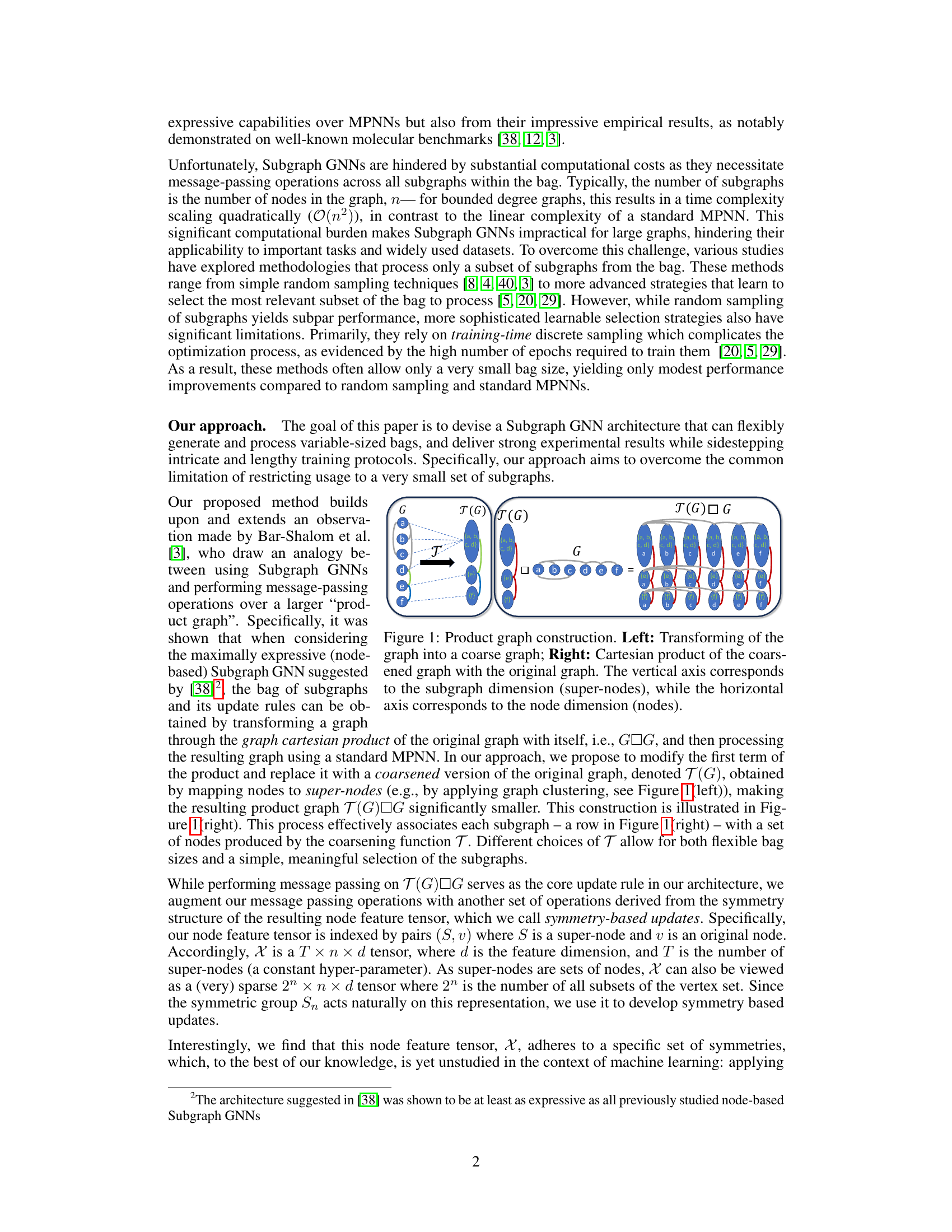
🔼 This figure illustrates the construction of the product graph used in the CS-GNN framework. The left panel shows how the original graph G is transformed into a coarsened graph T(G) by mapping nodes to super-nodes. The right panel shows the Cartesian product of T(G) and G, resulting in a product graph with a new connectivity structure. Each row in this product graph represents a subgraph, where the super-nodes from T(G) determine which nodes are included in each subgraph. This allows the model to process a variable number of subgraphs.
read the caption
Figure 1: Product graph construction. Left: Transforming of the graph into a coarse graph; Right: Cartesian product of the coarsened graph with the original graph. The vertical axis corresponds to the subgraph dimension (super-nodes), while the horizontal axis corresponds to the node dimension (nodes).
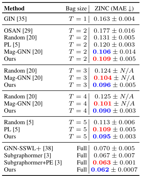
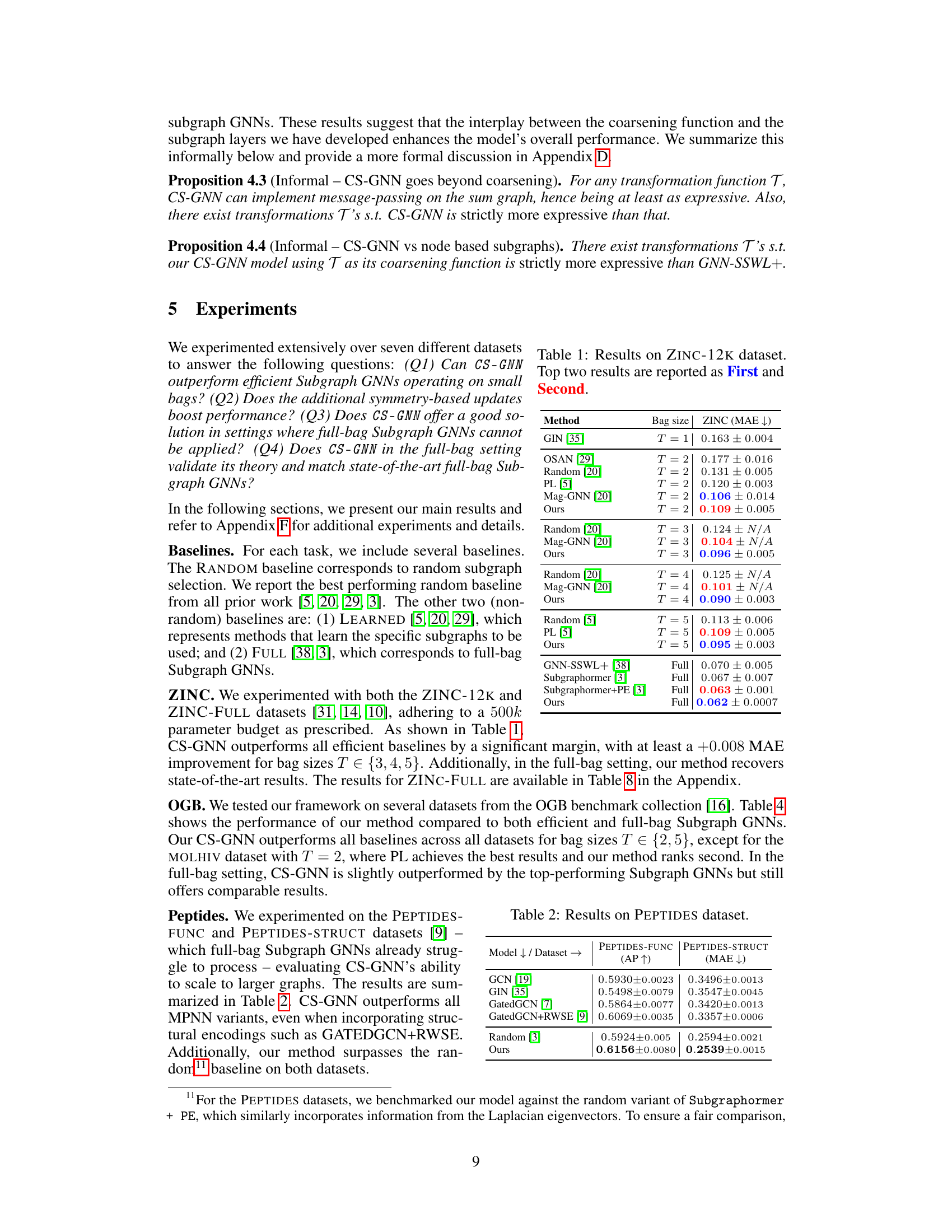
🔼 This table presents the results of the proposed CS-GNN model and several baseline models on the ZINC-12K dataset. The results are shown for different bag sizes (T), indicating the number of subgraphs considered. The table also includes the results of state-of-the-art full-bag Subgraph GNN models for comparison.
read the caption
Table 1: Results on ZINC-12K dataset. Top two results are reported as First and Second.
In-depth insights#
Equivariant Subgraph GNNs#
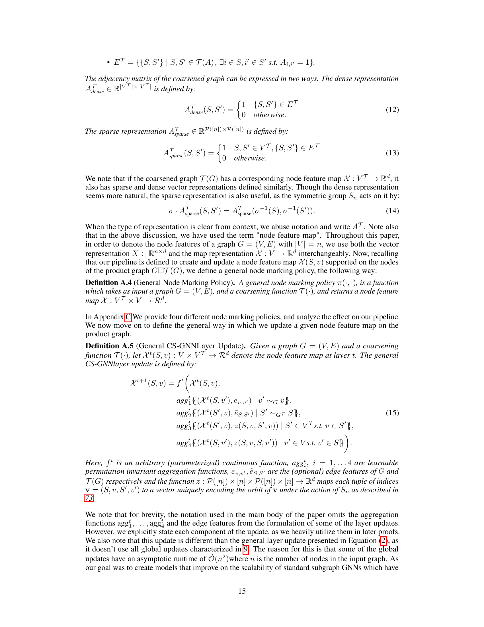
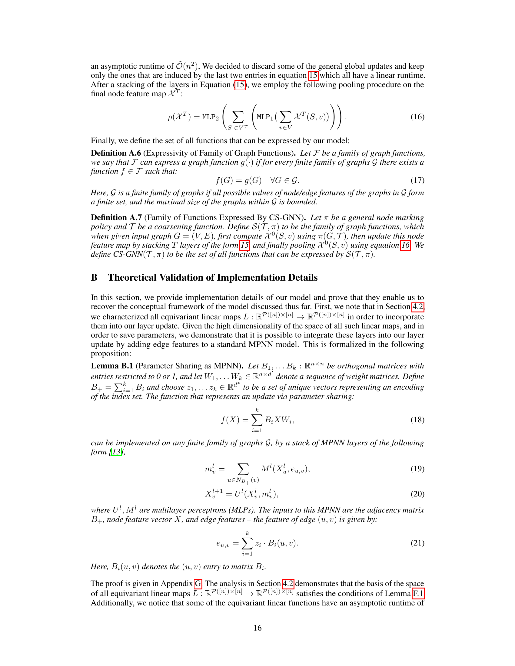
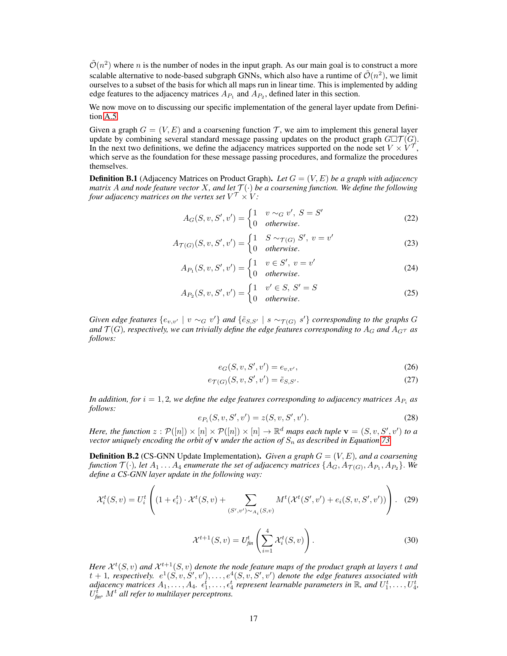
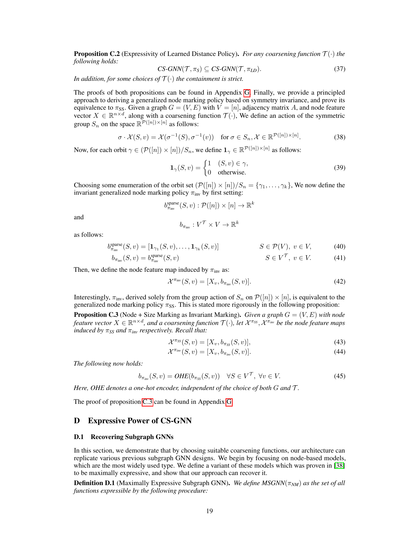
Equivariant Subgraph Graph Neural Networks (GNNs) represent a significant advancement in graph representation learning. They enhance the expressiveness of standard GNNs by operating on sets of subgraphs rather than the entire graph. This approach is particularly powerful because it allows the model to capture higher-order relationships and structural patterns often missed by traditional methods. The “equivariant” property is crucial, ensuring that the model’s predictions remain consistent even when the input graph undergoes transformations like node permutations. This invariance to symmetry is key for tasks requiring robust generalization, such as molecular property prediction where different representations of the same molecule should produce identical results. By leveraging the symmetries within the subgraph structures, equivariant subgraph GNNs achieve increased efficiency and accuracy compared to their non-equivariant counterparts.
Product Graph Approach#
A product graph approach in a research paper likely involves representing graph data as a product of two or more graphs, creating a higher-order structure that captures more complex relationships within the data. This approach is particularly useful when dealing with tasks that necessitate understanding subgraph structures, such as molecular property prediction or social network analysis. Constructing the product graph often involves graph operations like Cartesian product or Kronecker product, which combine the original graphs based on specific rules. The resulting product graph can then be analyzed using standard graph neural network techniques, or it can be processed using a custom designed method to effectively leverage the newly formed connections and properties of the product graph. The benefits include increased expressivity in modeling complex interactions and improved scalability by strategically reducing the size and complexity of the product graph. However, challenges include choosing the appropriate graph operations and managing the increased computational cost associated with processing large product graphs. A successful implementation requires careful selection of the original graphs and graph operations based on the characteristics of the problem domain and the desired level of complexity in the model.
Symmetry-Based Updates#
The heading ‘Symmetry-Based Updates’ hints at a crucial methodology in the paper. It suggests that the authors leverage inherent symmetries within their novel graph representation to improve model performance. This likely involves designing update rules that are equivariant or invariant under certain symmetry transformations of the graph. By respecting these symmetries, the model learns more generalizable features that aren’t tied to specific node or edge orderings, leading to better generalization and robustness. The specific symmetries utilized and the manner in which they are incorporated into the update rules are important to understand. Equivariant layers, which transform features consistently with graph symmetries, are probable components. The approach likely improves efficiency and expressivity by reducing redundant computations and capturing higher-order structural information not captured by standard message-passing. The theoretical analysis of the symmetry properties and the empirical demonstration of improved performance are critical aspects of this section’s contribution. Novel node marking strategies might interact with the symmetry-based updates for enhanced feature extraction and model expressivity. Overall, this section unveils a key innovation that distinguishes the proposed framework and warrants a thorough examination.
Coarsening Strategies#
Coarsening strategies are crucial for efficient Subgraph Graph Neural Networks (Subgraph GNNs). They determine how the original graph is simplified into a smaller representation, impacting the computational cost and expressiveness. Effective coarsening balances reduction in size with preservation of crucial structural information. Random coarsening is simple but often suboptimal. Learned coarsening methods offer adaptability but can be complex and require significant computational resources for training. The choice of coarsening strategy significantly affects the resulting Subgraph GNN’s performance, with a well-chosen strategy leading to enhanced expressiveness and scalability. A key aspect is the trade-off between the computational cost of generating and processing the coarsened graph, and the information loss due to simplification. Ideally, coarsening should prioritize the preservation of essential topological features while discarding redundant or less informative details, ultimately enhancing the Subgraph GNN’s efficiency and accuracy.
Scalability and Expressivity#
The inherent tension between scalability and expressivity is a central challenge in many machine learning domains, particularly graph neural networks (GNNs). Enhanced expressivity, often achieved through more complex architectures or higher-order interactions, frequently comes at the cost of reduced scalability, especially when dealing with large graphs. Subgraph GNNs, while offering improved expressivity by considering sets of subgraphs, often suffer from quadratic time complexity due to the need to process numerous subgraphs. This paper addresses this tradeoff by proposing a novel framework that leverages graph products and coarsening techniques. Graph coarsening effectively reduces the number of subgraphs, leading to improved scalability. Simultaneously, the framework exploits inherent symmetries within the product graph to design linear equivariant layers, thereby maintaining or even improving expressivity. The key contribution lies in this flexible and efficient approach that allows for handling variable-sized subsets of subgraphs, striking a balance between the desired properties.
More visual insights#
More on figures

🔼 This figure shows the performance comparison of different Subgraph GNN methods on the ZINC-12K dataset with varying numbers of subgraphs (bag sizes). The x-axis represents the bag size, and the y-axis represents the Mean Absolute Error (MAE), a measure of prediction accuracy. The results show that the proposed method consistently outperforms other methods, especially in scenarios with smaller bag sizes. It also performs competitively with state-of-the-art methods in the full bag setting.
read the caption
Figure 2: The performance landscape of Subgraph GNNs with varying number of subgraphs: Our method leads in the lower bag-size set, outperforming other approaches in nearly all cases. Additionally, our method matches the performance of state-of-the-art Subgraph GNNs in the full-bag setting. The full mean absolute error (MAE) scores along with standard deviations are available in Table 9 in the appendix.

🔼 This figure illustrates the construction of the product graph used in the proposed Subgraph GNN framework. The left panel shows how the original graph is transformed into a coarse graph by mapping nodes to super-nodes (clusters). The right panel shows the cartesian product of the coarse graph and the original graph, resulting in a new graph where rows represent subgraphs associated with clusters of nodes, and columns represent the original nodes. This product graph structure provides a new connectivity on which generalized message passing is performed, enabling flexible subgraph selection and efficient processing.
read the caption
Figure 1: Product graph construction. Left: Transforming of the graph into a coarse graph; Right: Cartesian product of the coarsened graph with the original graph. The vertical axis corresponds to the subgraph dimension (super-nodes), while the horizontal axis corresponds to the node dimension (nodes).

🔼 This figure visualizes the parameter sharing scheme for linear equivariant layers, comparing the proposed method with previous approaches. The left panel shows the weight matrix for the equivariant basis, while the right panel shows the bias vector for the invariant basis. The proposed method leverages symmetries to reduce the number of parameters significantly.
read the caption
Figure 3: Visualization via heatmaps (different colors correspond to different parameters) of the parameter-sharing scheme determined by symmetries for a graph with n = 6 nodes, zooming-in on the block which corresponds to sets of size two. Left: Visualization of the weight matrix for the equivariant basis B51,11;52,12 (a total of 35 parameters in the block). Right: Visualization of the bias vector for the invariant basis B (a total of 2 parameters in the block). Symmetry-based updates reduce parameters more effectively than previously proposed linear equivariant layers by treating indices as unordered tuples (see Appendix E.3 for a discussion).

🔼 This figure illustrates the construction of the product graph used in the CS-GNN framework. The left panel shows how the original graph is coarsened by mapping nodes to super-nodes. The right panel depicts the Cartesian product of the coarsened graph and the original graph, which results in a new connectivity structure where each row represents a subgraph associated with a set of nodes from the coarsened graph. This product graph forms the basis for generalized message passing in the CS-GNN.
read the caption
Figure 1: Product graph construction. Left: Transforming of the graph into a coarse graph; Right: Cartesian product of the coarsened graph with the original graph. The vertical axis corresponds to the subgraph dimension (super-nodes), while the horizontal axis corresponds to the node dimension (nodes).
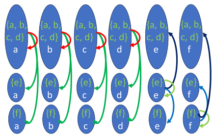
🔼 The figure illustrates the construction of a product graph used in the proposed Subgraph GNN framework. The left panel shows how an original graph is coarsened by mapping nodes to super-nodes, effectively clustering nodes. The right panel shows the Cartesian product of this coarsened graph with the original graph. Each row in the product graph represents a subgraph, and the entire structure visualizes how subgraphs are associated with node clusters rather than individual nodes, a key difference from prior approaches.
read the caption
Figure 1: Product graph construction. Left: Transforming of the graph into a coarse graph; Right: Cartesian product of the coarsened graph with the original graph. The vertical axis corresponds to the subgraph dimension (super-nodes), while the horizontal axis corresponds to the node dimension (nodes).
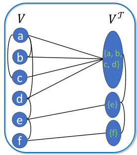
🔼 This figure illustrates the construction of the product graph used in the CS-GNN framework. The left panel shows the process of coarsening the original graph into a smaller graph by grouping nodes into super-nodes (clusters). The right panel illustrates the Cartesian product of the coarsened graph (vertical axis) with the original graph (horizontal axis). Each row in the right panel represents a subgraph in the Subgraph GNN framework, associating subgraphs with node clusters rather than individual nodes.
read the caption
Figure 1: Product graph construction. Left: Transforming of the graph into a coarse graph; Right: Cartesian product of the coarsened graph with the original graph. The vertical axis corresponds to the subgraph dimension (super-nodes), while the horizontal axis corresponds to the node dimension (nodes).

🔼 The figure illustrates the construction of a product graph used in the CS-GNN framework. The left panel shows a graph being coarsened, reducing the number of nodes to super-nodes. The right panel displays the Cartesian product of the original graph and its coarsened version, illustrating how subgraphs are associated with node clusters rather than individual nodes. Each row in the product graph represents a subgraph. This process allows for a flexible and efficient selection of subgraphs of any size for processing.
read the caption
Figure 1: Product graph construction. Left: Transforming of the graph into a coarse graph; Right: Cartesian product of the coarsened graph with the original graph. The vertical axis corresponds to the subgraph dimension (super-nodes), while the horizontal axis corresponds to the node dimension (nodes).
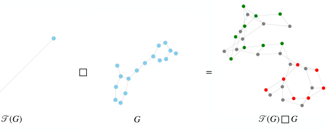
🔼 This figure illustrates the construction of the product graph used in the CS-GNN framework. The left panel shows how the original graph is coarsened by mapping nodes to super-nodes. The right panel shows the Cartesian product of this coarsened graph with the original graph. Each row in the right panel represents a subgraph, and the overall structure reveals a new connectivity structure used for generalized message passing. The vertical axis represents subgraph dimension (super-nodes), while the horizontal axis represents the node dimension (nodes).
read the caption
Figure 1: Product graph construction. Left: Transforming of the graph into a coarse graph; Right: Cartesian product of the coarsened graph with the original graph. The vertical axis corresponds to the subgraph dimension (super-nodes), while the horizontal axis corresponds to the node dimension (nodes).
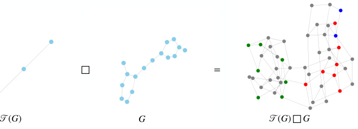
🔼 This figure illustrates the construction of the product graph used in the CS-GNN framework. The left panel shows how the original graph is coarsened by mapping nodes to super-nodes, forming a coarse graph. The right panel depicts the Cartesian product of the coarse graph and the original graph. Each row in the product graph represents a subgraph, where each subgraph is associated with a set of nodes determined by the coarsening function. The product graph construction is central to the method’s ability to generate and process variable-sized bags of subgraphs.
read the caption
Figure 1: Product graph construction. Left: Transforming of the graph into a coarse graph; Right: Cartesian product of the coarsened graph with the original graph. The vertical axis corresponds to the subgraph dimension (super-nodes), while the horizontal axis corresponds to the node dimension (nodes).

🔼 The figure illustrates the construction of the product graph used in the proposed Subgraph GNN framework. The left panel shows how the original graph is coarsened by grouping nodes into super-nodes. The right panel depicts the Cartesian product of the coarsened graph and the original graph. Each row in the right panel represents a subgraph, showing how the framework associates subgraphs with node clusters rather than individual nodes. The vertical axis represents the subgraph dimension (supernodes), while the horizontal axis represents the node dimension (nodes).
read the caption
Figure 1: Product graph construction. Left: Transforming of the graph into a coarse graph; Right: Cartesian product of the coarsened graph with the original graph. The vertical axis corresponds to the subgraph dimension (super-nodes), while the horizontal axis corresponds to the node dimension (nodes).

🔼 The figure illustrates the construction of the product graph used in the CS-GNN framework. The left panel shows how a graph is coarsened by grouping nodes into super-nodes. The right panel shows the Cartesian product of this coarsened graph with the original graph. Each row in the product graph represents a subgraph, and the overall structure highlights how subgraphs are associated with node clusters rather than individual nodes, a key aspect of the proposed method. The vertical and horizontal axes correspond to the subgraph and node dimensions respectively.
read the caption
Figure 1: Product graph construction. Left: Transforming of the graph into a coarse graph; Right: Cartesian product of the coarsened graph with the original graph. The vertical axis corresponds to the subgraph dimension (super-nodes), while the horizontal axis corresponds to the node dimension (nodes).
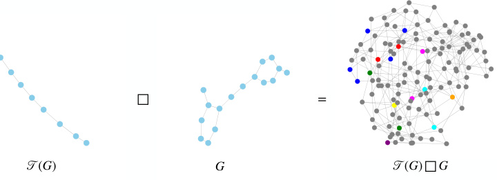
🔼 This figure illustrates the construction of the product graph used in the CS-GNN framework. The left panel shows the process of coarsening the original graph G, where nodes are mapped into super-nodes. The right panel shows the Cartesian product of the coarsened graph T(G) with the original graph G, resulting in a new graph T(G)□G. Each row in this product graph represents a subgraph, and the entire structure is used for message passing in the CS-GNN.
read the caption
Figure 1: Product graph construction. Left: Transforming of the graph into a coarse graph; Right: Cartesian product of the coarsened graph with the original graph. The vertical axis corresponds to the subgraph dimension (super-nodes), while the horizontal axis corresponds to the node dimension (nodes).
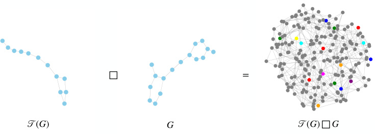
🔼 This figure illustrates the construction of the product graph used in the proposed Subgraph GNN framework. The left panel shows the original graph being coarsened, mapping multiple nodes into supernodes. The right panel shows the Cartesian product of this coarsened graph with the original graph, resulting in a new graph where each row represents a subgraph associated with a set of nodes from the coarsened graph. This product graph structure allows the method to efficiently handle a variable number of subgraphs and perform generalized message passing.
read the caption
Figure 1: Product graph construction. Left: Transforming of the graph into a coarse graph; Right: Cartesian product of the coarsened graph with the original graph. The vertical axis corresponds to the subgraph dimension (super-nodes), while the horizontal axis corresponds to the node dimension (nodes).

🔼 The figure illustrates how to construct a product graph. The left panel shows the process of transforming an original graph into a coarse graph by mapping nodes to supernodes (clusters). The right panel shows the cartesian product of the coarse graph and the original graph. This results in a new graph where each row represents a subgraph associated with a set of nodes from the coarsening, and the columns represent the original nodes. This product graph structure enables generalized message passing.
read the caption
Figure 1: Product graph construction. Left: Transforming of the graph into a coarse graph; Right: Cartesian product of the coarsened graph with the original graph. The vertical axis corresponds to the subgraph dimension (super-nodes), while the horizontal axis corresponds to the node dimension (nodes).
More on tables
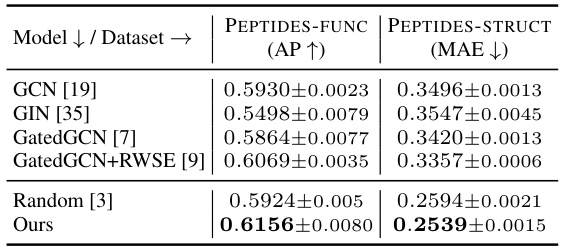
🔼 This table presents the results of experiments conducted on two PEPTIDES datasets: PEPTIDES-FUNC (multi-label graph classification) and PEPTIDES-STRUCT (multi-task regression). The table compares the performance of the proposed CS-GNN method against several baseline models, including GCN, GIN, GatedGCN, and GatedGCN+RWSE. The results are shown in terms of Average Precision (AP) for PEPTIDES-FUNC and Mean Absolute Error (MAE) for PEPTIDES-STRUCT. The CS-GNN model outperforms all baseline models on both datasets, demonstrating its effectiveness in handling large graph datasets.
read the caption
Table 2: Results on PEPTIDES dataset. Top two results are reported as First and Second.

🔼 This table presents the ablation study results for the impact of symmetry-based updates on the performance of the CS-GNN model. It shows the mean absolute error (MAE) achieved on the ZINC-12K dataset for different bag sizes (T) with and without the symmetry-based updates. The results demonstrate that the symmetry-based updates significantly improve the model’s performance across all bag sizes.
read the caption
Table 3: Ablation study.
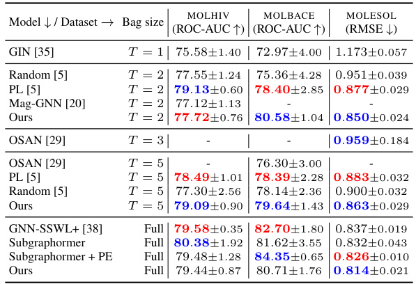
🔼 This table presents the results of experiments conducted on seven datasets from the Open Graph Benchmark (OGB) collection. The table compares the performance of the proposed CS-GNN model against several baseline methods across different bag sizes (number of subgraphs processed) and the full bag setting. For each dataset and bag size, it shows the performance metrics (ROC-AUC for MOLHIV, MOLBACE, and RMSE for MOLESOL). The results highlight the flexibility and performance gains achieved by the CS-GNN model.
read the caption
Table 4: Results on OGB datasets. The top two results are reported as First and Second.

🔼 This table presents eight graph datasets used for evaluating the proposed model, along with key characteristics such as the number of graphs, average number of nodes and edges, directionality (directed or undirected), prediction task (regression, classification), and the metric used for evaluation (e.g., Mean Absolute Error, AUROC, Root Mean Squared Error). The datasets represent diverse applications of graph learning and include various sizes and complexities.
read the caption
Table 5: Overview of the graph learning datasets.

🔼 This table presents the chosen hyperparameters for the CS-GNN model across various datasets and bag sizes. It includes hyperparameters like learning rate, embedding size, number of layers, epochs, batch size, dropout rate, Laplacian dimension, and SPD dimension, showing the specific values selected for each experiment. These settings are crucial for reproducibility of the results presented in the paper.
read the caption
Table 7: Chosen Hyperparameters for CS-GNN.

🔼 This table presents the chosen hyperparameters for the CS-GNN model across various datasets and bag sizes. The hyperparameters include the number of layers, learning rate, embedding size, number of epochs, batch size, dropout rate, Laplacian dimension, and SPD dimension. The choices of hyperparameters were made through a hyperparameter search process, details of which can be found in Appendix F.3 of the paper. Note that the Laplacian dimension and SPD dimension parameters relate to the coarsening process used to control the number of subgraphs processed.
read the caption
Table 7: Chosen Hyperparameters for CS-GNN.
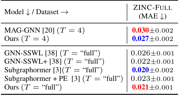
🔼 This table compares the performance of different models on the ZINC-FULL dataset, using a parameter budget of 500k. The models are evaluated based on their Mean Absolute Error (MAE). The best-performing model for each bag size (T) is highlighted in blue, and the second best in red. The table helps illustrate the relative performance of different Subgraph GNNs, specifically comparing the proposed method against state-of-the-art techniques, both in settings where a small subset of subgraphs is used and the full set is used.
read the caption
Table 8: Comparison over the ZINC-FULL molecular dataset under 500k parameter budget. The best performing method is highlighted in blue, while the second best is highlighted in red.
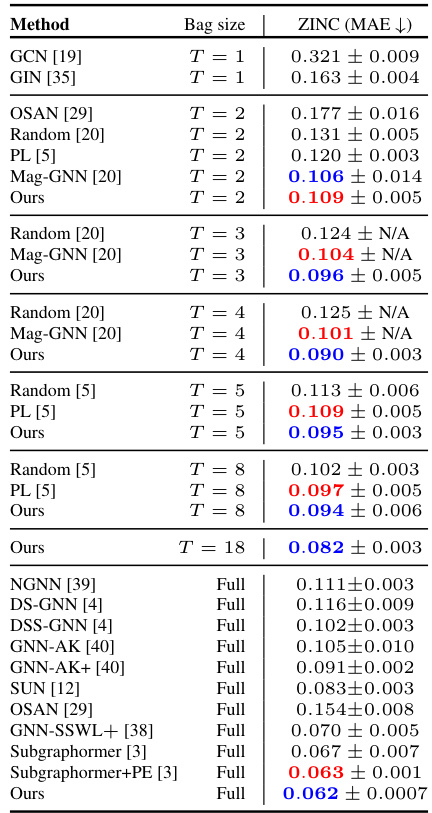
🔼 This table presents the results of the proposed CS-GNN model and several baseline methods on the ZINC-12K dataset for different bag sizes (number of subgraphs). The results show Mean Absolute Error (MAE) values for each model, indicating its performance in predicting molecular properties. The table highlights that CS-GNN outperforms other methods, especially in smaller bag sizes, demonstrating its effectiveness in handling various numbers of subgraphs.
read the caption
Table 1: Results on ZINC-12K dataset. Top two results are reported as First and Second.

🔼 This table presents a runtime comparison of different methods on the ZINC-12K dataset. For each method, it shows the training time for a single epoch and the inference time on the test set, both measured in milliseconds. The Mean Absolute Error (MAE) is also included for context.
read the caption
Table 10: Run time comparison over the ZINC-12K dataset. Time taken at train for one epoch and at inference on the test set. All values are in milliseconds.
Full paper#
