TL;DR#
Deep learning’s reliance on massive datasets presents challenges due to data curation difficulties. Existing data point selection (DPS) methods, often based on computationally expensive bi-level optimization, struggle with efficiency and theoretical shortcomings. This limitation hinders the training of large models, particularly in resource-intensive domains like language processing.
This paper proposes BADS (Bayesian Approach to Data Selection), a novel Bayesian method for DPS. BADS frames DPS as a posterior inference problem within a Bayesian model. It uses stochastic gradient Langevin dynamics for efficient parameter and weight inference, exhibiting convergence even with minibatches. Experimental results across vision and language tasks, including large language models, demonstrate BADS’ superior efficiency and scalability compared to existing BLO methods.
Key Takeaways#
Why does it matter?#
This paper is important because it introduces a novel Bayesian approach to data point selection (DPS), a critical problem in deep learning. The proposed method, BADS, is significantly more efficient than existing methods based on bi-level optimization. It scales effectively to large language models, demonstrating its practical applicability. The work opens up new avenues for automating per-task optimization and data curation, addressing a major bottleneck in training modern AI systems.
Visual Insights#
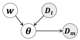
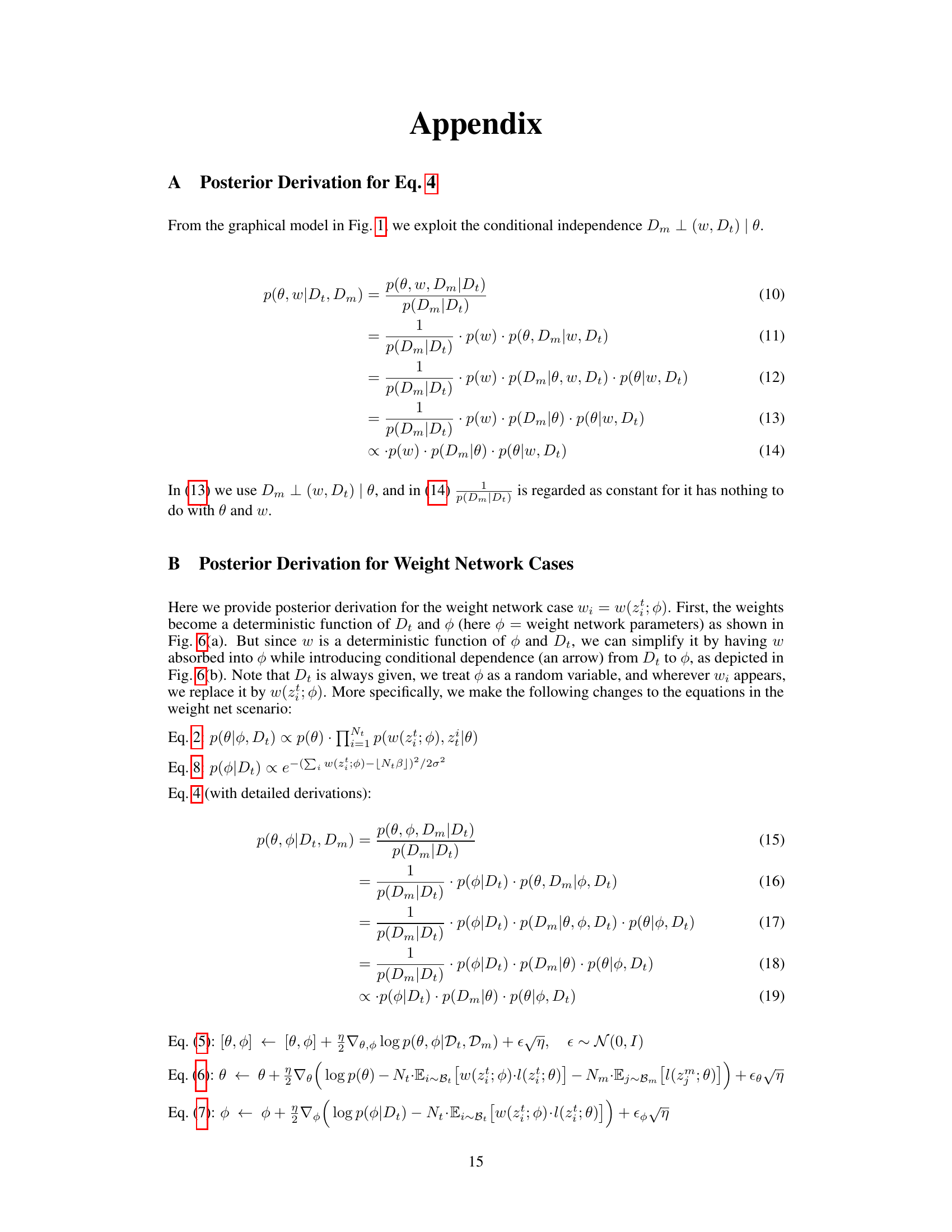
🔼 This figure presents the graphical model for the Bayesian Approach to Data Selection (BADS) method proposed in the paper. The model involves three main components: the instance-wise weights (w), which represent the importance of each data point in the uncurated training data (Dt), the model parameters (θ) of the neural network, and the curated meta-dataset (Dm). The shaded nodes (Dt and Dm) represent observed data, acting as evidence. The unshaded nodes (w and θ) are unobserved random variables, which the model infers. The model assumes that the weights w influence the prior distribution of the model parameters θ, given the uncurated data Dt. Then, the model parameters θ determine the likelihood of generating the curated meta-dataset Dm. The overall goal is to infer the posterior distribution p(θ, w|Dt, Dm) by performing Bayesian inference.
read the caption
Figure 1: Graphical model for BADS. Shaded nodes, representing curated (Dm) and uncurated (Dt) data, are evidence. Unshaded nodes, including model θ and instance weights w, are random variables.
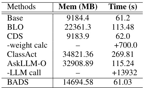
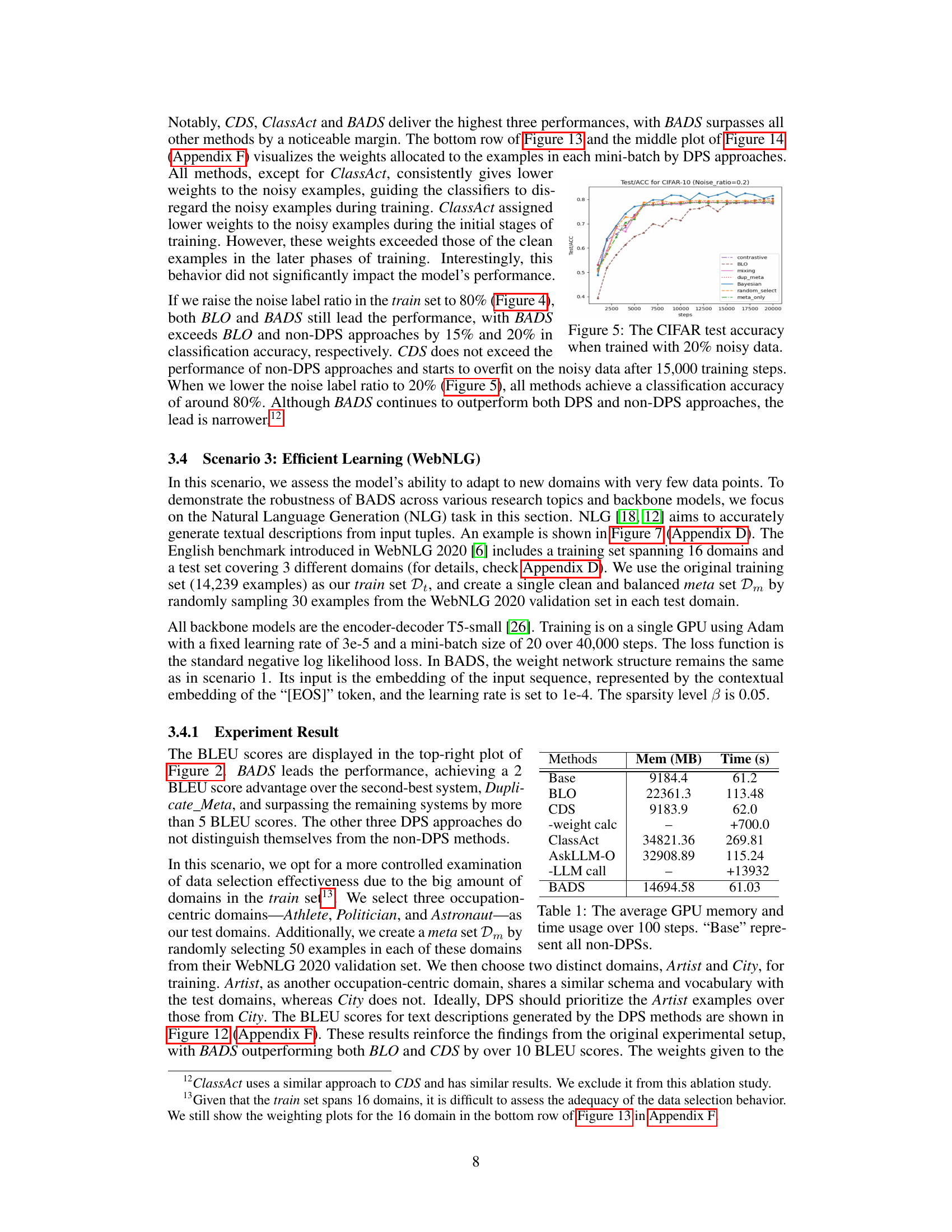
🔼 This table presents a comparison of GPU memory and time usage across different methods for data point selection in the WebNLG task. The ‘Base’ row represents the memory and time usage for traditional methods (non-DPS), providing a baseline for comparison. The table shows that BADS and CDS have similar memory and time usage to the baseline methods. However, BLO and AskLLM-O require substantially more time, while ClassAct requires significantly more memory and time than other methods. Note that CDS and AskLLM-O require additional time to calculate weights and perform LLM calls respectively.
read the caption
Table 1: The average GPU memory and time usage over 100 steps. 'Base' represent all non-DPSs.
In-depth insights#
Bayesian DPS#
A Bayesian approach to data point selection (DPS) offers a compelling alternative to traditional methods. Instead of relying on computationally expensive bi-level optimization, a Bayesian framework elegantly frames DPS as a posterior inference problem. This involves inferring both the neural network parameters and instance-wise weights, offering advantages in terms of efficiency and scalability. The use of stochastic gradient Langevin dynamics for sampling enables efficient posterior inference, even with large datasets. This approach provides a clear convergence guarantee, a significant improvement over the complexities inherent in bi-level optimization. The method also shows promise in handling various DPS challenges, such as noise, class imbalance, and data curation, within a unified framework. Empirical results demonstrate its effectiveness across vision and language domains, further highlighting its potential for practical applications, especially when dealing with large language models and instruction fine-tuning datasets.
SGLD Sampling#
Stochastic Gradient Langevin Dynamics (SGLD) sampling is a crucial technique in the paper’s Bayesian approach to data point selection. SGLD cleverly combines stochastic gradient descent with added Gaussian noise to sample from the intractable posterior distribution of model parameters and instance weights. This approach is particularly valuable because it avoids the computationally expensive calculations and convergence issues associated with traditional bi-level optimization methods. The update equations in SGLD are strikingly similar to standard SGD, making them computationally efficient and easy to implement. Furthermore, SGLD’s inherent ability to handle minibatches elegantly addresses a key limitation of previous methods which struggle with theoretical and practical convergence when dealing with minibatches. The efficiency of SGLD is especially beneficial when scaling to large language models, where computational costs are often prohibitive. However, it is important to note that the efficiency does come at the cost of requiring careful tuning of hyperparameters and careful handling of the potential for sparsity and convergence issues.
Proof-of-Concept#
A Proof-of-Concept section in a research paper serves as a crucial bridge between theoretical claims and practical validation. It demonstrates the feasibility of the proposed approach by presenting compelling empirical evidence. A strong Proof-of-Concept showcases results that are not only positive but also statistically significant, ideally using multiple metrics to offer a holistic view. The selection of datasets is vital, ensuring they are representative and appropriately challenging, while rigorous methodology avoids biases and ensures repeatability. The section should clearly highlight the novel aspects demonstrated by the proposed method and compare its performance against established baselines. Strong visuals such as graphs and tables are essential for effectively communicating results and facilitating analysis. Ultimately, a well-executed Proof-of-Concept builds confidence in the core claims of the paper and paves the way for future developments and broader applications.
Method Limits#
A research paper’s ‘Method Limits’ section would critically analyze the constraints and shortcomings of the proposed methodology. It might discuss computational cost, scalability issues with large datasets or models, and the reliance on specific assumptions (e.g., data distribution, noise levels) that might not hold in real-world applications. The section should acknowledge limitations in generalizability, perhaps due to the use of specific datasets or the choice of evaluation metrics. A thoughtful analysis would also consider the reproducibility of results, noting factors that could affect the repeatability of experiments (e.g., hardware requirements, random seeds). Finally, the authors would ideally suggest avenues for future work, addressing the identified limitations to improve the robustness and applicability of the method.
Future Work#
The authors acknowledge several avenues for future research. Improving hyperparameter tuning is crucial, potentially through Bayesian optimization to automate the selection of parameters like sparsity level (β) and impact constants (ρ). Addressing the high GPU memory demands is another key area; they suggest investigating techniques to load only necessary weights, reducing memory footprint. Exploring alternative sampling methods beyond SGLD is also proposed to potentially improve efficiency and convergence. Finally, a more in-depth exploration of the weight network’s architecture, including the use of more sophisticated network designs, is noted to further enhance the model’s performance and generalization capabilities. These improvements will lead to better scalability and make the model more robust and practical for various applications.
More visual insights#
More on figures
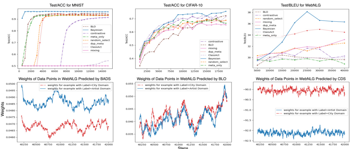
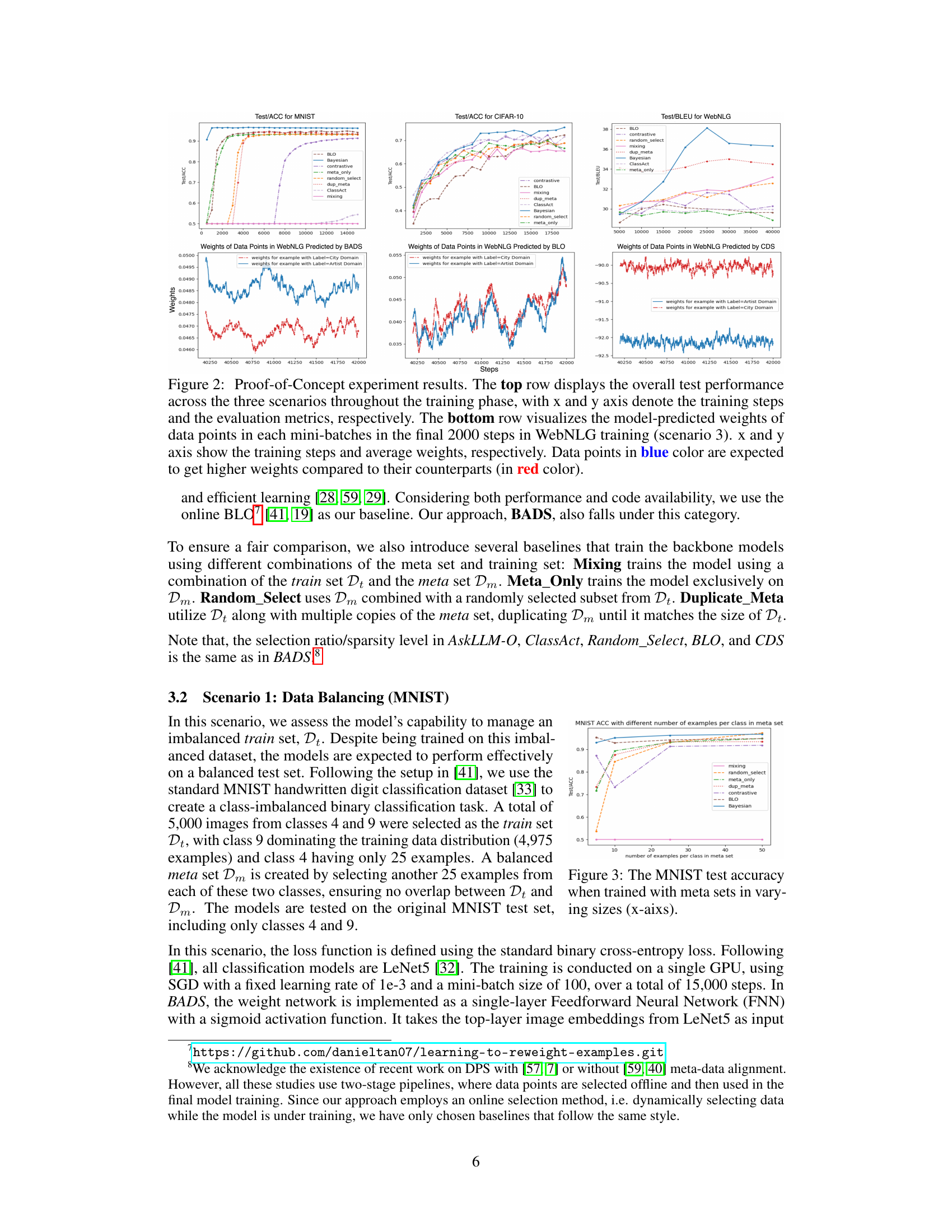
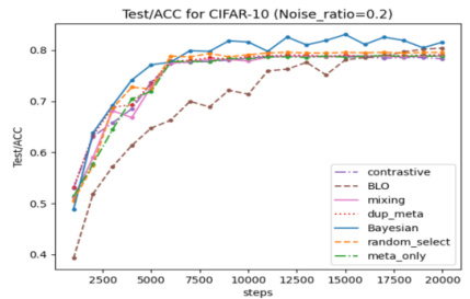
🔼 The figure shows the experimental results of the proposed method (BADS) and several baselines on three different scenarios: Data Balancing (MNIST), Data Denoising (CIFAR-10), and Efficient Learning (WebNLG). The top row displays the overall test performance for each scenario, comparing BADS to various baselines including BLO, CDS, ClassAct, mixing, etc. The bottom row visualizes the weights assigned by BADS to data points in the WebNLG scenario. The visualization shows that BADS assigns higher weights to specific data points, which is expected to improve performance.
read the caption
Figure 2: Proof-of-Concept experiment results. The top row displays the overall test performance across the three scenarios throughout the training phase, with x and y axis denote the training steps and the evaluation metrics, respectively. The bottom row visualizes the model-predicted weights of data points in each mini-batches in the final 2000 steps in WebNLG training (scenario 3). x and y axis show the training steps and average weights, respectively. Data points in blue color are expected to get higher weights compared to their counterparts (in red color).
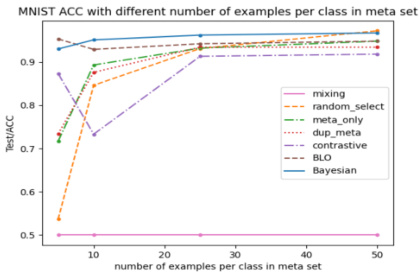
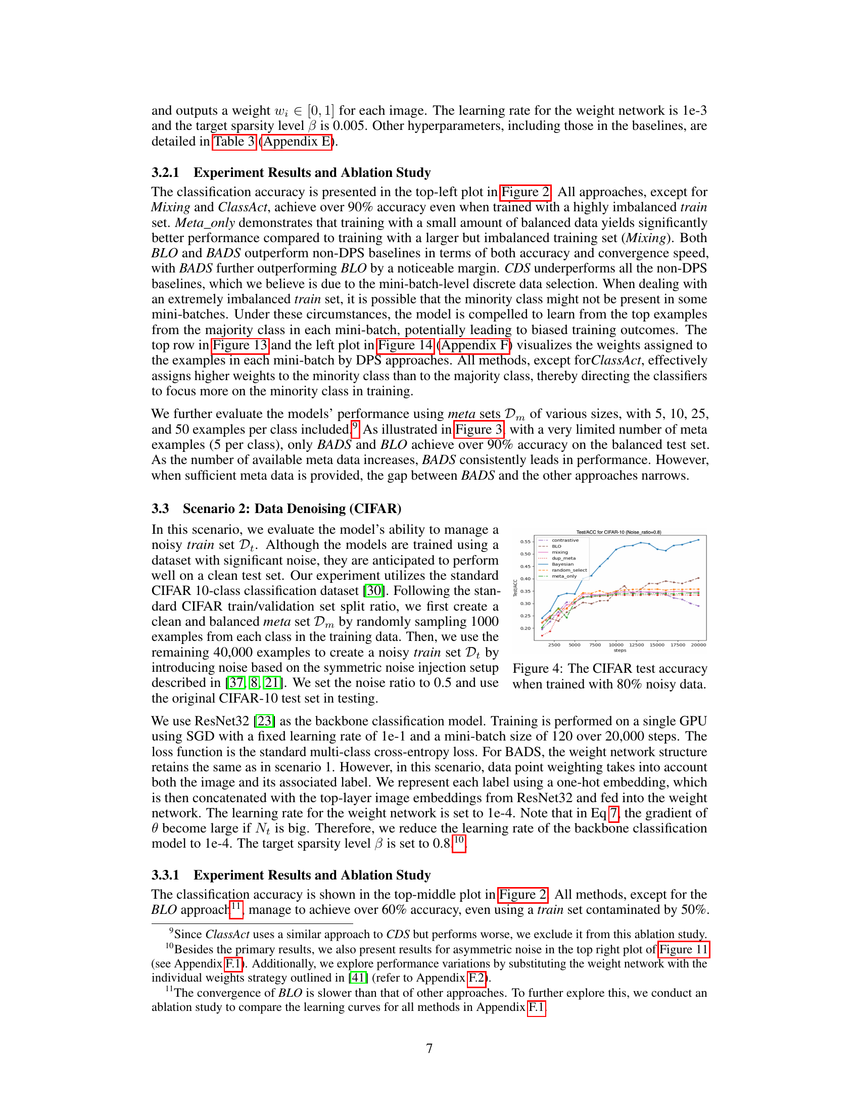
🔼 This figure shows the MNIST test accuracy with different sizes of meta sets. The x-axis represents the number of examples per class in the meta set, while the y-axis shows the test accuracy. Each line represents a different data selection method: mixing, random_select, meta_only, dup_meta, contrastive, BLO, and Bayesian. The plot illustrates how the test accuracy changes as the size of the meta set increases for each method. It highlights the performance differences between various data selection techniques when dealing with imbalanced datasets. Notably, the Bayesian approach consistently outperforms other methods, especially with limited meta data.
read the caption
Figure 3: The MNIST test accuracy when trained with meta sets in varying sizes (x-aixs).
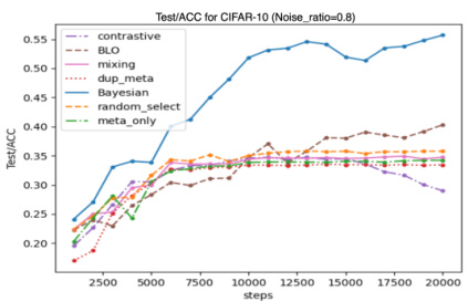
🔼 The figure shows the test performance of different data selection methods across three scenarios (data balancing, denoising, and efficient learning) throughout the training process. The bottom part visualizes how the model assigns weights to data points in each minibatch for WebNLG training. Points predicted to be more important are highlighted in blue, while those predicted to be less important are in red.
read the caption
Figure 2: Proof-of-Concept experiment results. The top row displays the overall test performance across the three scenarios throughout the training phase, with x and y axis denote the training steps and the evaluation metrics, respectively. The bottom row visualizes the model-predicted weights of data points in each mini-batches in the final 2000 steps in WebNLG training (scenario 3). x and y axis show the training steps and average weights, respectively. Data points in blue color are expected to get higher weights compared to their counterparts (in red color).
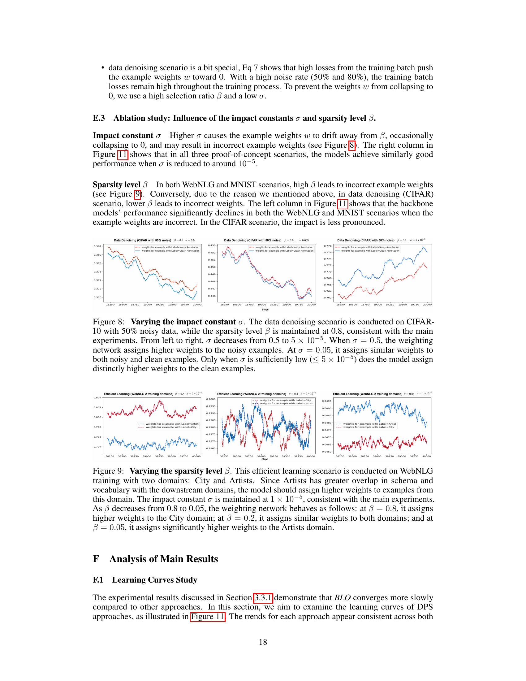
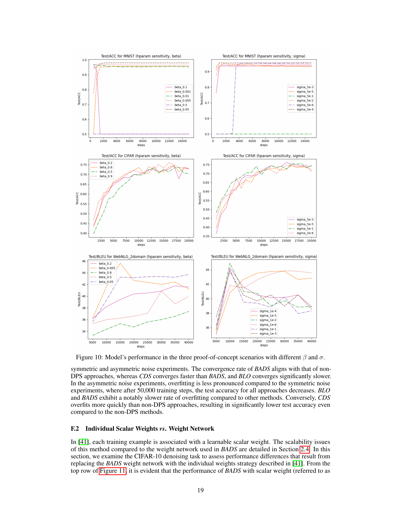
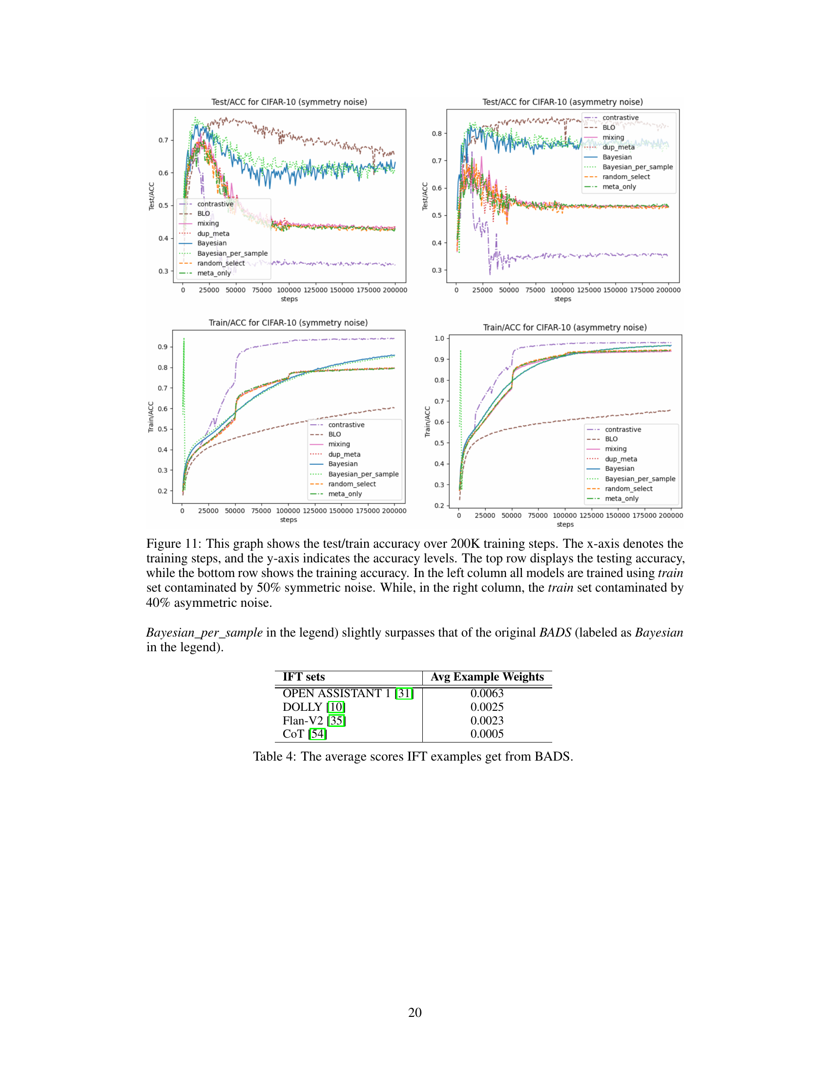
🔼 This figure displays the test accuracy for three different scenarios (MNIST, CIFAR, and WebNLG) across various hyperparameter settings for β (sparsity level) and σ (impact constant). It visualizes how these hyperparameters affect the model’s performance and convergence speed across different DPS (Data Point Selection) approaches and compares them to non-DPS baselines. Each subplot represents a different scenario, with the x-axis showing training steps and the y-axis showing test accuracy. The results illustrate the impact of β and σ on the models’ performance, convergence rate, and overall ability to handle imbalanced, noisy, and limited data.
read the caption
Figure 10: Model’s performance in the three proof-of-concept scenarios with different β and σ.

🔼 This figure shows the graphical model used in the Bayesian Approach to Data Point Selection (BADS) method. The shaded nodes represent the curated meta dataset (Dm) and uncurated training dataset (Dt). These are considered as evidence in the Bayesian model. The unshaded nodes represent the model parameters (θ) and instance-wise weights (w). These are random variables to be inferred. The model illustrates how the instance weights (w), given the uncurated data (Dt), influence the prior distribution of model parameters (θ). In turn, the model parameters (θ) influence the likelihood of generating the meta dataset (Dm). The goal is to infer the posterior distribution of both model parameters (θ) and instance weights (w) given both the curated and uncurated datasets.
read the caption
Figure 1: Graphical model for BADS. Shaded nodes, representing curated (Dm) and uncurated (Dt) data, are evidence. Unshaded nodes, including model θ and instance weights w, are random variables.
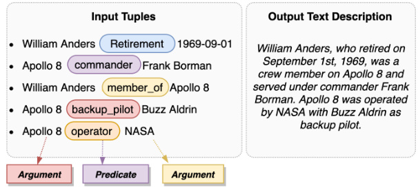
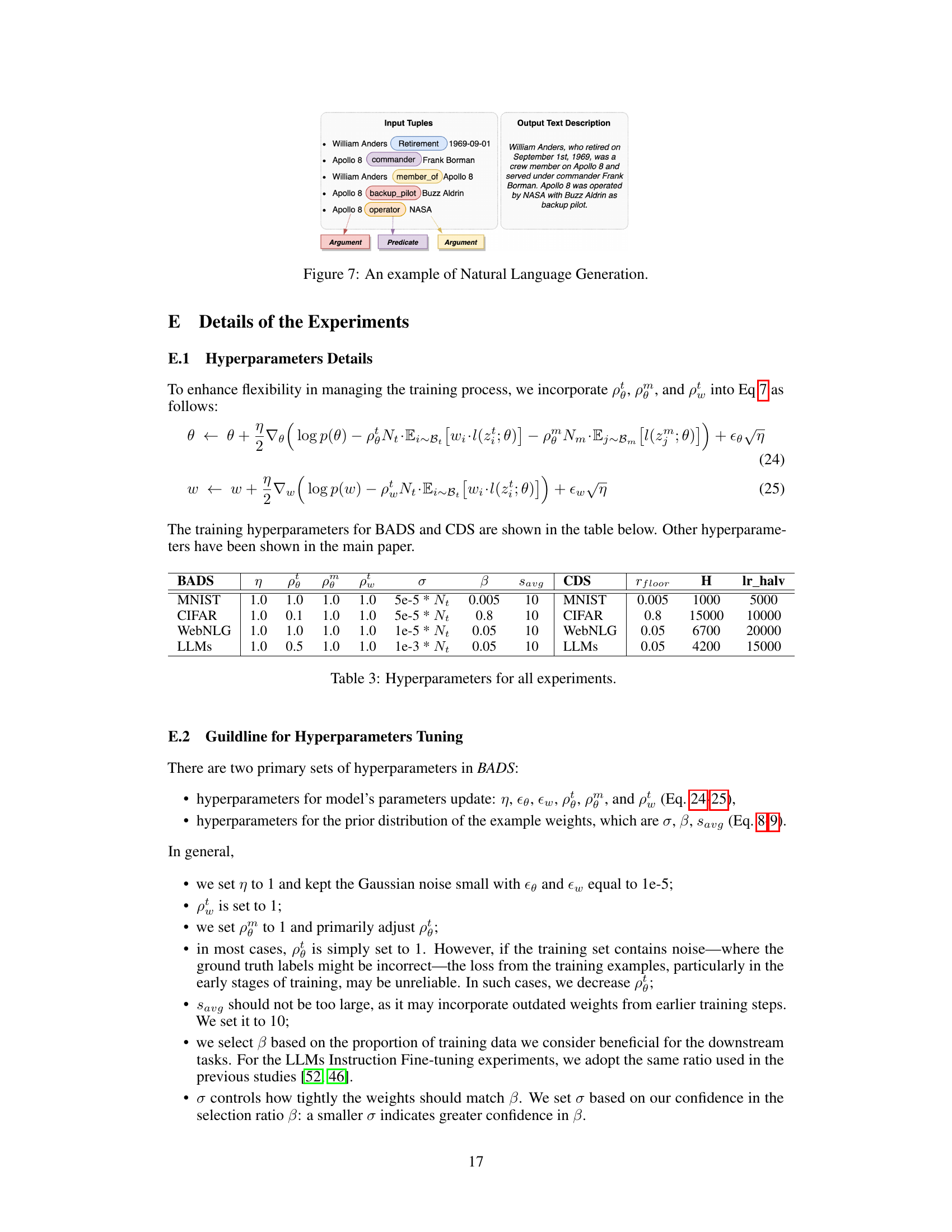
🔼 The figure shows an example of how the WebNLG task works. Input tuples consist of multiple (argument, predicate, argument) triplets, which are then used to generate a natural language text description. This example illustrates the process of transforming structured data into a coherent textual narrative.
read the caption
Figure 7: An example of Natural Language Generation.

🔼 This figure displays the test accuracy across three scenarios (MNIST, CIFAR, WebNLG) using different values of β (sparsity level) and σ (impact constant) in the BADS method. Each subplot shows the test accuracy curves for various values of β or σ, allowing for an analysis of their individual and combined influence on model performance across different tasks. The results reveal the sensitivity of the BADS method to these hyperparameters and how their optimization is crucial for achieving optimal model performance. The consistent trends across all three scenarios help to support the robustness and general applicability of the BADS approach.
read the caption
Figure 10: Model's performance in the three proof-of-concept scenarios with different β and σ.

🔼 The figure displays the performance of different models (BADS, BLO, CDS, and other baselines) across three scenarios: Data Balancing (MNIST), Data Denoising (CIFAR), and Efficient Learning (WebNLG). Each scenario is tested with various hyperparameters (β and σ). The x-axis shows training steps, and the y-axis shows the evaluation metric (accuracy or BLEU score). The plots show how the hyperparameters affect the performance of the models. For example, the impact of varying the hyperparameters on model performance in the three proof-of-concept scenarios is illustrated.
read the caption
Figure 10: Model's performance in the three proof-of-concept scenarios with different β and σ.
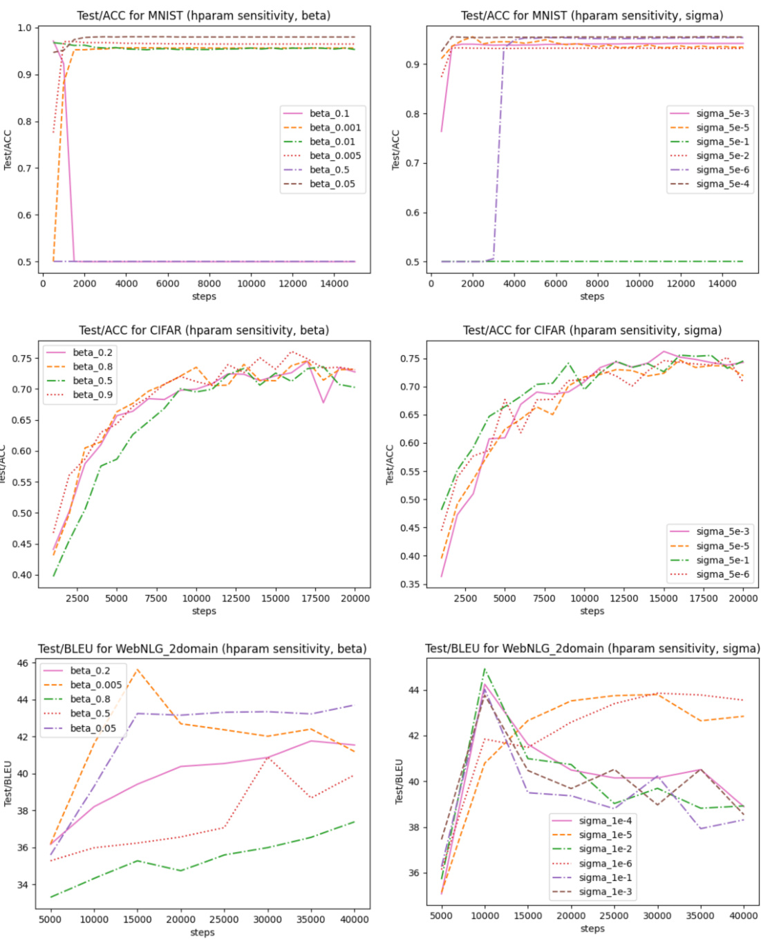
🔼 This figure presents the performance of the proposed method (BADS) and baselines across three scenarios (Data Balancing, Data Denoising, Efficient Learning) with varying hyperparameters β (sparsity level) and σ (impact constant). It shows the test accuracy/BLEU score over training steps for each scenario and different values of β and σ, illustrating the sensitivity of the model’s performance to these hyperparameters and the relative effectiveness of BADS in comparison to the other approaches. The results are separated into plots showing the effect of changing β while keeping σ constant and vice-versa.
read the caption
Figure 10: Model's performance in the three proof-of-concept scenarios with different β and σ.
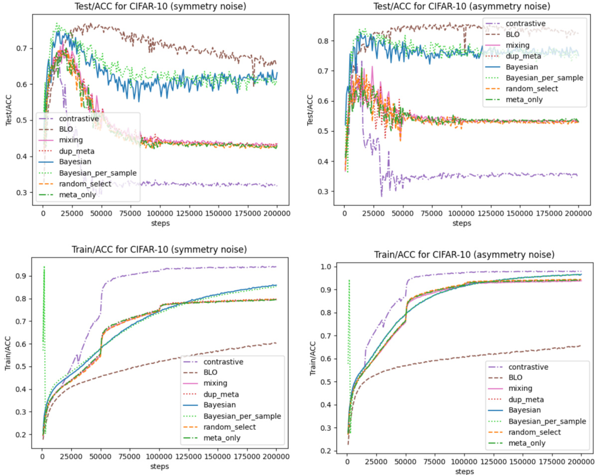
🔼 This figure displays the model’s performance across three scenarios (MNIST, CIFAR, and WebNLG) with varying β (sparsity level) and σ (impact constant). It visually compares the performance of the BADS model against multiple baselines under different hyperparameter settings. The trends shown illustrate the sensitivity of the model’s performance to these hyperparameters and help to understand the effect of different data selection strategies.
read the caption
Figure 10: Model's performance in the three proof-of-concept scenarios with different β and σ.
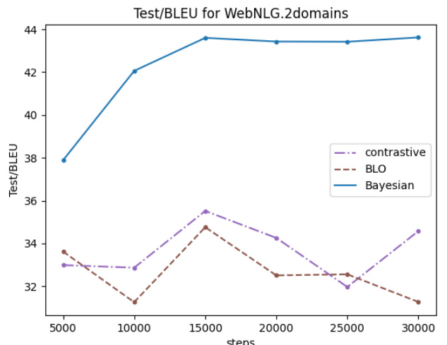
🔼 This figure shows the performance of the models in three scenarios (MNIST, CIFAR, WebNLG) with different values of β (sparsity level) and σ (impact constant). It illustrates how these hyperparameters affect the model’s convergence speed and overall accuracy. The plots compare the model’s test accuracy over the course of training, demonstrating the effect of the hyperparameters.
read the caption
Figure 10: Model's performance in the three proof-of-concept scenarios with different β and σ.
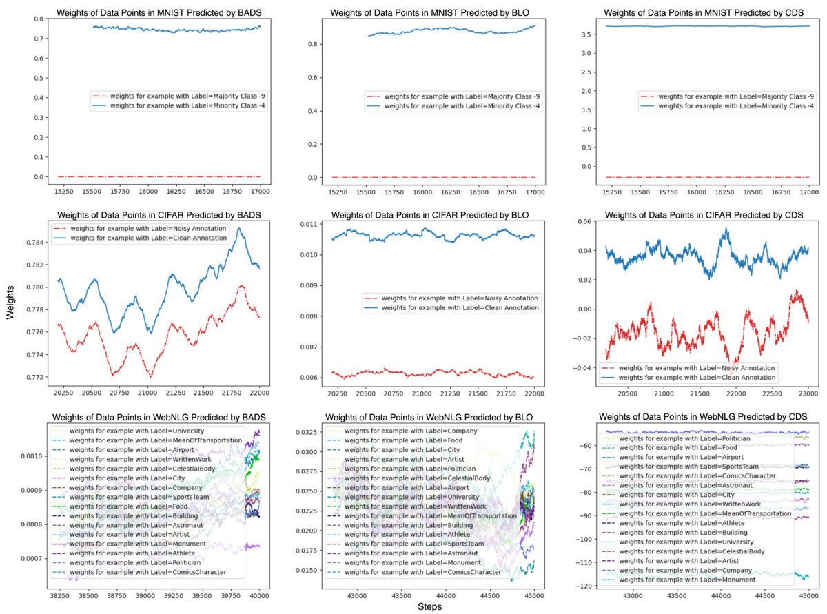
🔼 This figure provides supplementary results from three proof-of-concept experiments showing the average weights assigned to data points in mini-batches during the final stages of training. The plots show, for each of three methods (BADS, BLO, and CDS), the weights assigned to data points for the MNIST (data balancing), CIFAR (data denoising), and WebNLG (efficient learning) tasks, highlighting the differences in how the three methods prioritize data points.
read the caption
Figure 13: Proof-of-Concept experiment supplementary results. All plots illustrate the average weights of data points within mini-batches during the last 2000 training steps, with the x-axis representing the training steps and the y-axis showing the average weights. Classes depicted in blue are expected to receive higher weights compared to those in red. The top row displays the MNIST experiments from scenario 1, the middle row shows the CIFAR experiments from scenario 2, and the bottom row features the WebNLG experiments from scenario 3. The left, middle, and right columns correspond to BADS, BLO, and CDS, respectively.

🔼 This figure provides supplementary results for the three proof-of-concept experiments (data balancing, data denoising, and efficient learning) described in the paper. Each row shows the average weights assigned to different data points within mini-batches over the last 2000 training steps for one experiment. Blue data points are expected to have higher weights than red points. The three rows represent MNIST, CIFAR, and WebNLG experiments respectively; the columns represent BADS, BLO, and CDS algorithms. The visualization helps understand how each algorithm assigns weights to different data points in the different scenarios.
read the caption
Figure 13: Proof-of-Concept experiment supplementary results. All plots illustrate the average weights of data points within mini-batches during the last 2000 training steps, with the x-axis representing the training steps and the y-axis showing the average weights. Classes depicted in blue are expected to receive higher weights compared to those in red. The top row displays the MNIST experiments from scenario 1, the middle row shows the CIFAR experiments from scenario 2, and the bottom row features the WebNLG experiments from scenario 3. The left, middle, and right columns correspond to BADS, BLO, and CDS, respectively.
More on tables
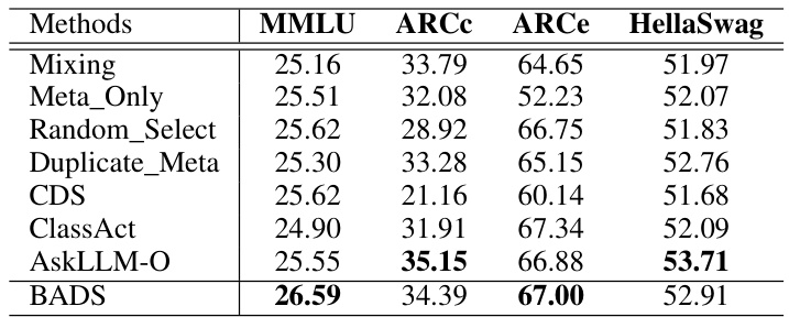
🔼 This table presents the test accuracy results for various Large Language Models (LLMs) evaluated on four popular benchmarks: MMLU, ARCC, ARCe, and HellaSwag. The models were trained using different data selection methods, including a baseline (‘Mixing’) representing standard Instruction Fine-Tuning (IFT). The ‘Checkpoint selection’ method used next token prediction accuracy. The table compares the performance of different data selection approaches against the standard IFT approach, highlighting the effectiveness of different strategies in improving LLM performance.
read the caption
Table 2: Test accuracy of LLMs across four popular benchmarks in eval-harness [17]. Checkpoint selection is using next token prediction accuracy as the selection metric. Mixing represents standard IFT.

🔼 This table lists the hyperparameter settings used in the experiments for different tasks and models. It shows the values for various parameters used in the Bayesian Data Point Selection (BADS) and Contrastive Data Selection (CDS) methods, such as learning rates (η), impact constants (ρθ, ρφ, ρw), noise standard deviation (σ), sparsity level (β), running average step (Savg), floor ratio for CDS (rfloor), hidden layer size (H), and lr_halfv which likely refers to a learning rate adjustment. Each row represents a different experiment (MNIST, CIFAR, WebNLG, LLMs).
read the caption
Table 3: Hyperparameters for all experiments.

🔼 This table shows the average weights assigned by the BADS model to examples from different Instruction Fine-tuning (IFT) datasets. It highlights the relative importance the model assigns to each dataset in the fine-tuning process, suggesting that some datasets contribute more significantly to the overall performance than others. These weights inform the data selection strategy used by BADS to optimize the fine-tuning process.
read the caption
Table 4: The average scores IFT examples get from BADS.
Full paper#
