TL;DR#
Risk-constrained reinforcement learning (RCRL) aims to ensure safety by explicitly handling risk-measure-based constraints. However, the nonlinearity of risk measures makes it challenging to achieve both convergence and optimality. Existing methods often only guarantee local convergence, limiting their effectiveness. This poses a significant challenge for deploying RL agents in safety-critical scenarios where worst-case outcomes must be avoided.
To tackle this challenge, the authors propose a novel spectral risk measure-constrained RL algorithm called Spectral-Risk-Constrained Policy Optimization (SRCPO). SRCPO leverages the duality of spectral risk measures through a bilevel optimization framework. The outer problem optimizes dual variables derived from the risk measures, while the inner problem finds an optimal policy for given dual variables. The algorithm is the first to guarantee convergence to an optimum in the tabular setting and demonstrates state-of-the-art performance in continuous control tasks, consistently outperforming existing methods.
Key Takeaways#
Why does it matter?#
This paper is important because it addresses a critical challenge in risk-constrained reinforcement learning (RCRL): achieving both convergence and optimality in the presence of nonlinear risk measures. It proposes a novel algorithm, SRCPO, which guarantees convergence to a global optimum in tabular settings and demonstrates superior performance in continuous control tasks. This significantly advances the field of safe RL, enabling more reliable and efficient deployment of RL agents in safety-critical applications.
Visual Insights#
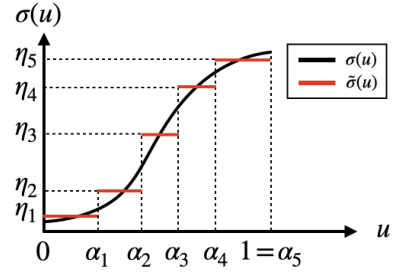
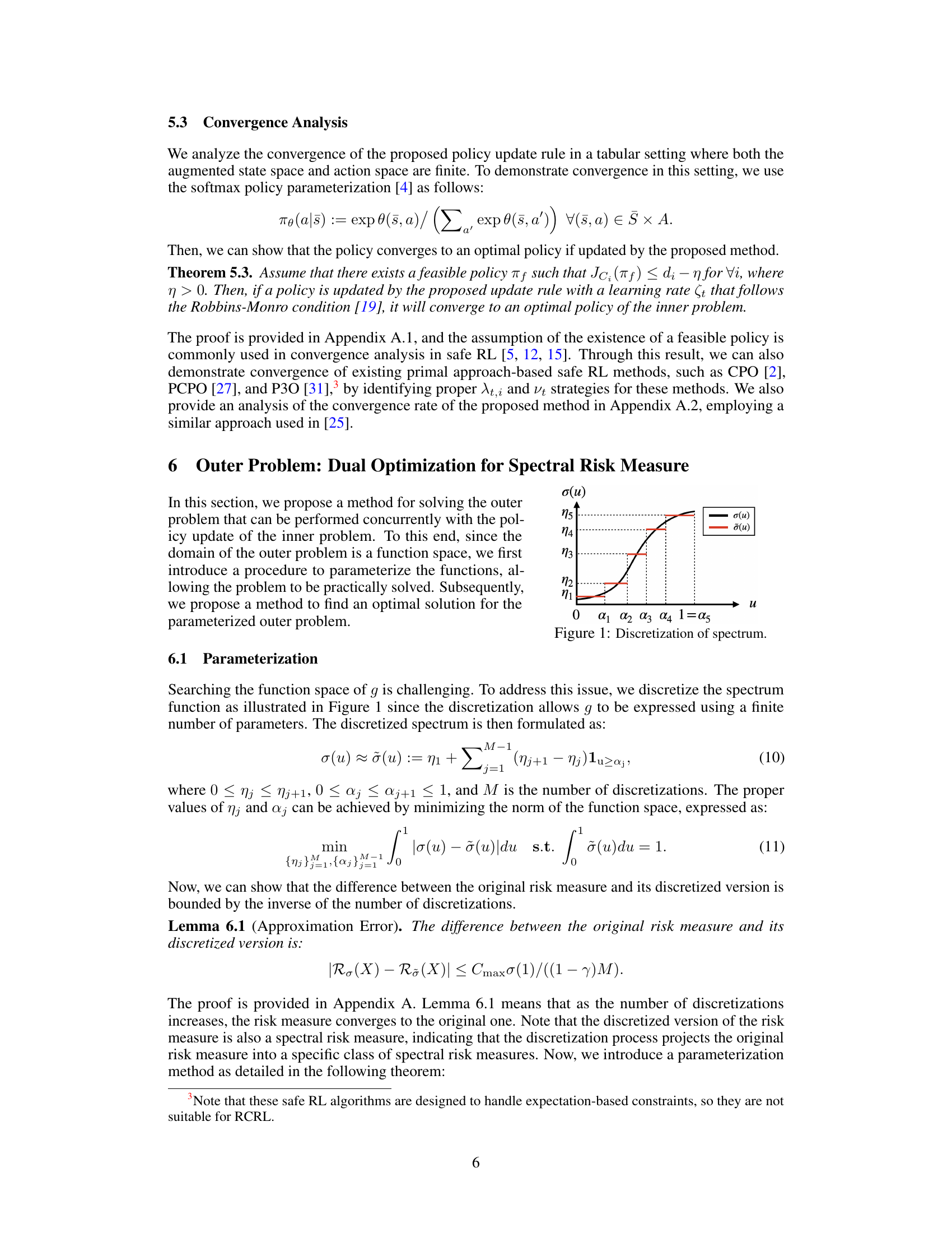
🔼 This figure illustrates the discretization of the spectrum function σ(u) used in spectral risk measures. The original spectrum (black line) is approximated by a piecewise constant function ỡ(u) (red line). The approximation uses a finite number of parameters, simplifying the optimization process in the outer problem of the SRCPO algorithm. The horizontal axis represents the cumulative probability u (from 0 to 1) and the vertical axis represents the spectrum value σ(u). The red lines show the piecewise constant approximation of the spectrum function, using M=5 discretized segments.
read the caption
Figure 1: Discretization of spectrum.

🔼 This table presents the architectural details of the neural networks used in the paper. It specifies the number of hidden layers, activation functions (LeakyReLU and Linear), and the output layer activation function (Linear for policy and reward critics, and SoftPlus for cost critics). Additionally, the number of quantiles and ensembles used in the quantile regression distributional critic are provided for the reward and cost critics.
read the caption
Table 1: Details of network structures.
In-depth insights#
Risk-Aware RL#
Risk-aware reinforcement learning (RL) tackles the crucial challenge of balancing reward maximization with risk mitigation. Standard RL often overlooks the potential for catastrophic failures, focusing solely on expected rewards. Risk-aware RL addresses this by explicitly incorporating risk measures into the RL framework. This involves defining risk metrics (e.g., variance, Value at Risk (VaR), Conditional Value at Risk (CVaR)), which quantify the uncertainty associated with different actions or policies. The goal is to learn policies that achieve high expected rewards while keeping the risk within acceptable limits, thus ensuring system robustness and safety. Different approaches exist for integrating risk into RL, including constraint-based methods (restricting risk below a threshold), penalty-based methods (adding a risk penalty to the reward function), and risk-sensitive methods (directly optimizing a risk-sensitive objective function). The choice of risk measure significantly impacts the resulting policy, as different measures capture different aspects of risk. Furthermore, computational challenges arise from the often non-convex nature of risk measures, requiring sophisticated optimization techniques for efficient learning. The field is expanding rapidly, driven by the need for safe and reliable RL applications in diverse domains, including robotics, finance, and healthcare.
SRCPO Algorithm#
The SRCPO algorithm, a novel approach to risk-constrained reinforcement learning, tackles the challenges of nonlinearity in risk measures by employing a bilevel optimization framework. The outer level optimizes dual variables derived from the spectral risk measure’s dual representation, while the inner level focuses on discovering an optimal policy given these variables. A key innovation is the use of novel risk value functions exhibiting linearity in policy performance differences. This linearity enables the algorithm to guarantee convergence to an optimal policy, a significant advancement over existing methods that often only achieve local optimality. Furthermore, the algorithm’s efficiency is enhanced by modeling a distribution over dual variables, allowing the optimization process to bypass direct computation in the high-dimensional space, making the method more practical for continuous control tasks. The overall performance is superior in continuous control experiments compared to other risk-constrained methods. The algorithm’s theoretical guarantees and strong empirical results suggest it’s a promising advancement in safe reinforcement learning.
Convergence Proof#
A rigorous convergence proof is crucial for establishing the reliability and trustworthiness of any machine learning algorithm. In the context of reinforcement learning, a convergence proof demonstrates that the algorithm’s policy will reliably approach an optimal solution. This is particularly important in safety-critical applications where unpredictable behavior can have severe consequences. A successful convergence proof would typically involve demonstrating that the algorithm’s updates monotonically improve the policy’s performance, measured by a suitable metric, and that this improvement continues until it converges to a solution that satisfies specified optimality conditions. This often necessitates analyzing the algorithm’s dynamics, including the interaction between its different components, such as the policy update rule and the constraint handling mechanism, and proving that the process remains stable and converges to a desired state. The complexity of the proof will highly depend on the characteristics of the RL algorithm, particularly the complexity of its update rules and the nature of the constraints. Simpler algorithms may allow for more straightforward proofs, while more sophisticated algorithms may require more involved techniques from areas like optimization theory or stochastic processes. The type of convergence (e.g., global vs. local convergence) is also a critical aspect to consider, with global convergence being the stronger and more desirable result. In the absence of a global convergence guarantee, the practical performance of the algorithm becomes more reliant on experimental validation, which may not fully capture its behavior in all possible situations.
Empirical Results#
An effective ‘Empirical Results’ section should present a clear and concise summary of experimental findings. It should begin by outlining the experimental setup, including datasets used, evaluation metrics, and baseline methods. Visualizations are crucial: well-designed graphs and tables effectively communicate results. The discussion should highlight key findings, focusing on trends and patterns rather than individual data points. Statistical significance should be explicitly addressed, with appropriate error bars or statistical tests reported to support the validity of observed differences. A comparison to state-of-the-art baselines is vital to demonstrating the method’s effectiveness. Limitations of the experiments should also be acknowledged and discussed. Finally, the section needs to connect the experimental outcomes to the paper’s main claims, showing how the results support or challenge the presented hypotheses. A strong ‘Empirical Results’ section builds credibility and strengthens the overall impact of the research.
Future Works#
The paper’s ‘Future Works’ section could fruitfully explore extending the proven convergence and optimality results from the tabular setting to more complex scenarios. Addressing continuous state and action spaces is crucial for real-world applications. This might involve investigating approximate dynamic programming techniques or advanced function approximation methods to maintain theoretical guarantees. Another important direction would be to scale the algorithm to handle high-dimensional problems more effectively, perhaps by incorporating advanced optimization strategies or parallelization techniques. Furthermore, empirical evaluation on a wider range of tasks and benchmark environments would strengthen the paper’s impact and demonstrate the algorithm’s robustness and generalizability. Finally, a deeper investigation into the effect of different risk measures and their parameterizations could provide valuable insights into selecting the most appropriate measure for specific applications and explore novel risk-sensitive reward shaping methods.
More visual insights#
More on figures

🔼 This figure displays the training curves for two legged robot locomotion tasks (quadrupedal and bipedal). It compares several reinforcement learning algorithms (SRCPO, CPPO, CVaR-CPO, SDAC, WCSAC-D, and SDPO) across four metrics: reward sum, and three cost rates (Cost Rate 1, 2, 3). Each algorithm’s performance is shown as a line plot, with shaded areas representing standard deviations. Horizontal lines represent the constraint thresholds for cost rates. The figure illustrates the relative performance of each algorithm in achieving high rewards while satisfying multiple constraints.
read the caption
Figure 2: Training curves of the legged robot locomotion tasks. The upper graph shows results for the quadrupedal robot, and the lower one is for the bipedal robot. The solid line in each graph represents the average of each metric, and the shaded area indicates the standard deviation scaled by 0.5. The results are obtained by training each algorithm with five random seeds.

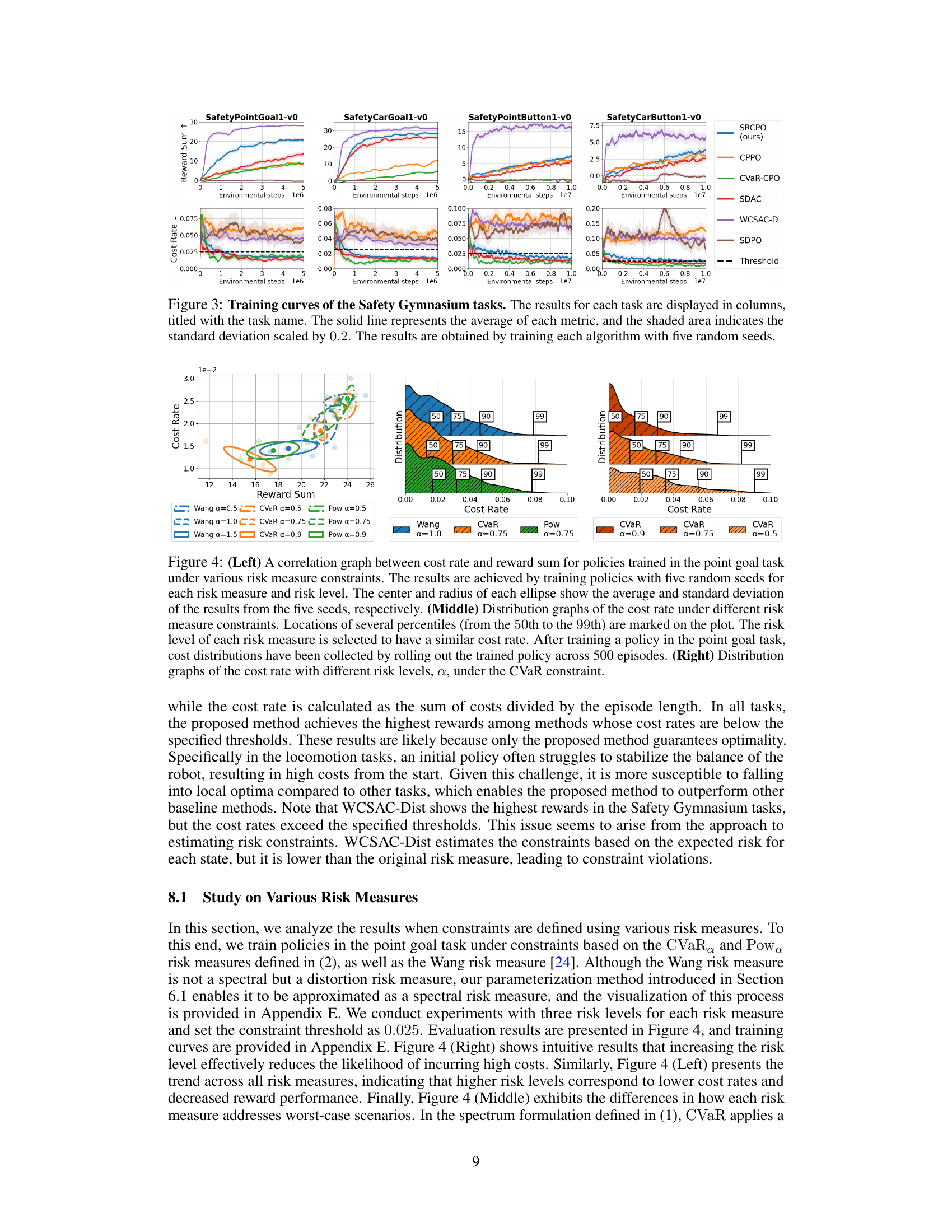
🔼 Training curves for four Safety Gymnasium tasks (point goal, car goal, point button, car button) comparing the proposed Spectral-Risk-Constrained Policy Optimization (SRCPO) method to four other safe reinforcement learning algorithms (CPPO, CVaR-CPO, SDAC, WCSAC-D, SDPO). The plots show reward sum and cost rate over training time (environmental steps). Shaded regions represent standard deviation (scaled by 0.2). Each algorithm was run with five random seeds.
read the caption
Figure 3: Training curves of the Safety Gymnasium tasks. The results for each task are displayed in columns, titled with the task name. The solid line represents the average of each metric, and the shaded area indicates the standard deviation scaled by 0.2. The results are obtained by training each algorithm with five random seeds.

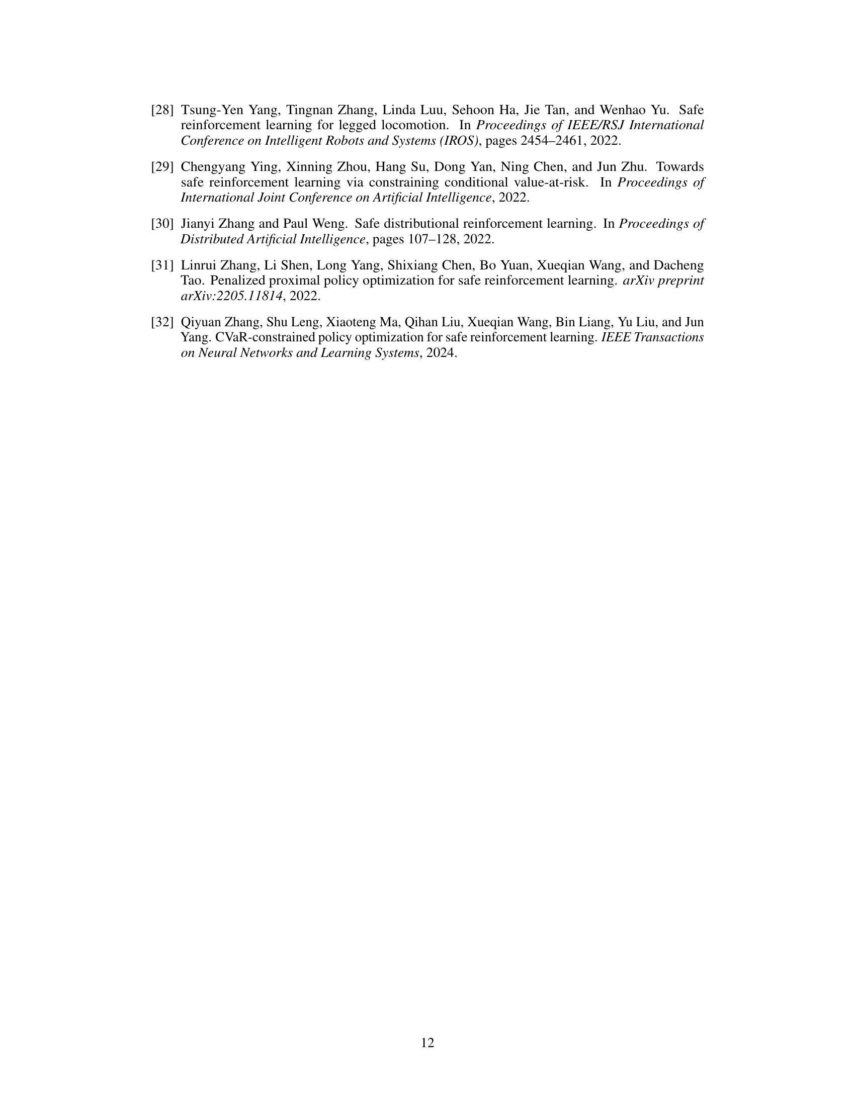
🔼 This figure shows the correlation between cost rate and reward sum for different risk measures (Wang, CVaR, Pow) and risk levels (alpha). The left panel displays ellipses representing the mean and standard deviation of the cost rate and reward sum for policies trained under each condition. The middle panels show the cost rate distributions, illustrating the effect of each risk measure and its associated risk level on the distribution of cost rates. The right panel shows the distribution of cost rates under different risk levels for CVaR specifically.
read the caption
Figure 4: (Left) A correlation graph between cost rate and reward sum for policies trained in the point goal task under various risk measure constraints. The results are achieved by training policies with five random seeds for each risk measure and risk level. The center and radius of each ellipse show the average and standard deviation of the results from the five seeds, respectively. (Middle) Distribution graphs of the cost rate under different risk measure constraints. Locations of several percentiles (from the 50th to the 99th) are marked on the plot. The risk level of each risk measure is selected to have a similar cost rate. After training a policy in the point goal task, cost distributions have been collected by rolling out the trained policy across 500 episodes. (Right) Distribution graphs of the cost rate with different risk levels, a, under the CVaR constraint.

🔼 The figure shows four different environments used in the experiments. (a) and (b) are the Safety Gymnasium environments, where a point robot or a car-like robot needs to reach a goal position or press a button without colliding with obstacles. (c) and (d) are the legged robot locomotion environments, where a quadrupedal or a bipedal robot needs to track a desired velocity while maintaining balance and avoiding falls.
read the caption
Figure 5: Rendered images of the Safety Gymnasium and the legged robot locomotion tasks.

🔼 This figure visualizes the original and discretized spectrum functions of the Wang risk measure for three different risk levels (α = 0.5, 1.0, 1.5). The original spectrum, a continuous function, is compared against its discretized counterpart, which is a piecewise constant function obtained through the discretization process described in Section 6.1 of the paper. This process approximates the continuous spectrum with a finite number of parameters, making it computationally feasible to solve the optimization problem. The plots show how the discretized spectrum closely approximates the original, especially for lower values of u (cumulative distribution function). The differences are more noticeable at higher u values where the original spectrum function increases sharply.
read the caption
Figure 6: Visualization of the spectrum function of the Wang risk measure and the discretized results.

🔼 This figure visualizes the original and discretized spectrum functions for the Wang risk measure at three different risk levels (α = 0.5, 1.0, 1.5). The discretization, a crucial step in the proposed SRCPO algorithm, approximates the original spectrum function using a finite number of parameters for computational tractability. The plots show how the discretized spectrum closely follows the shape of the original spectrum, demonstrating the effectiveness of the discretization method.
read the caption
Figure 6: Visualization of the spectrum function of the Wang risk measure and the discretized results.
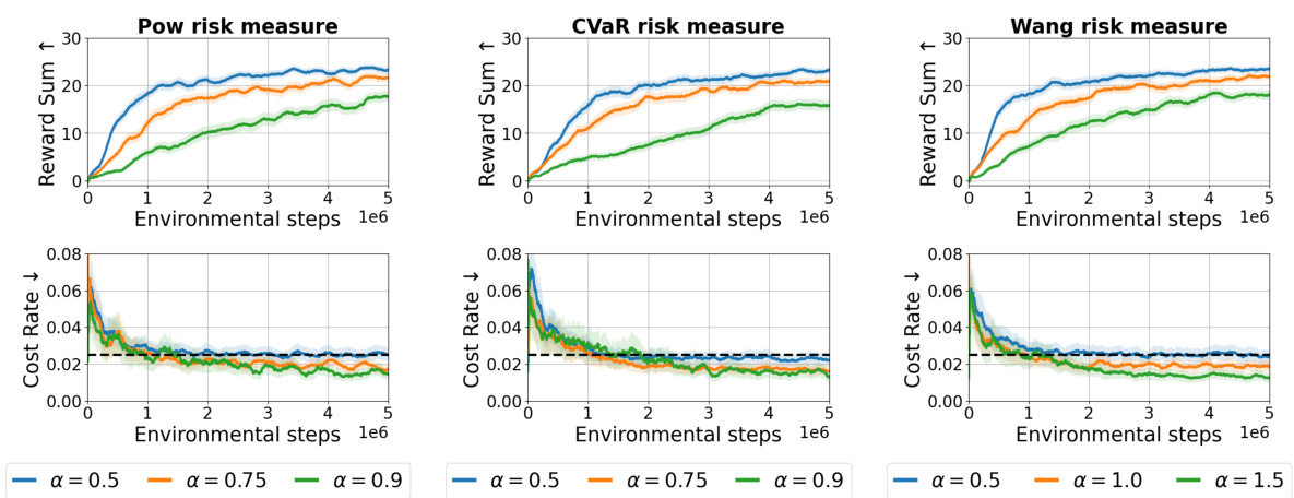
🔼 This figure shows the training curves for the point goal task using different risk measures (Pow, CVaR, and Wang) and different risk levels (α). Each measure’s performance is plotted across five random seeds, with the solid line indicating the average reward and cost rate, and shaded area representing standard deviation. This illustrates the impact of different risk measures and levels on the reward achieved while maintaining cost constraints.
read the caption
Figure 8: Training curves of the point goal task with different risk levels and risk measures. Each column shows the results on the risk measure whose name appears in the plot title. The solid line in each graph represents the average of each metric, and the shaded area indicates the standard deviation scaled by 0.2. The results are obtained by training algorithms with five random seeds.
More on tables
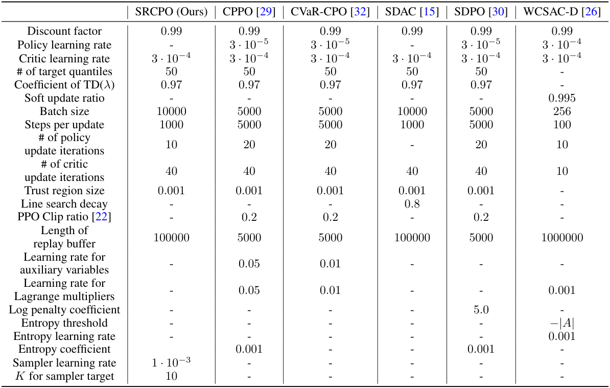
🔼 This table lists the hyperparameter settings used in the experiments for all the algorithms, including the proposed SRCPO method and several baseline methods. It covers various aspects of algorithm configuration, such as learning rates, batch sizes, numbers of updates, and parameters specific to certain algorithms like the trust region size for CPO and the entropy coefficient for SAC. The table helps clarify the experimental setup and ensure reproducibility of results.
read the caption
Table 2: Description on hyperparameter settings.

🔼 This table presents the averaged training time for six different safe reinforcement learning algorithms on the point goal task of the safety gymnasium. The training time is measured in hours, minutes, and seconds and averaged over five separate training runs for each algorithm. The purpose is to provide a comparison of the computational efficiency of different methods.
read the caption
Table 3: Training time for the point goal task averaged over five runs.

🔼 The table shows the results of the discretization of the Wang and Pow risk measures for different risk levels (α = 0.5, 1.0, 0.75, 0.9). For each risk measure and risk level, the table provides the optimized values of the parameters {nj} and {aj} for the discretized spectrum, as defined in equation (10). These parameters are obtained by minimizing the distance between the original spectrum function and its discretized version, as described in the paper.
read the caption
Table 4: Discretization results.
Full paper#
