TL;DR#
Model reconstruction attacks exploit counterfactual explanations to steal machine learning models, posing a security threat. Existing methods often suffer from decision boundary shifts, especially with one-sided counterfactuals. This paper proposes Counterfactual Clamping Attack (CCA) which utilizes a unique loss function to improve model reconstruction accuracy using only one-sided counterfactuals.
CCA addresses decision boundary shifts by treating counterfactuals differently, improving fidelity. The paper presents novel theoretical relationships between reconstruction error and counterfactual queries, using polytope theory for convex boundaries and probabilistic guarantees for ReLU networks. Experiments across multiple datasets show improved fidelity with CCA compared to existing approaches.
Key Takeaways#
Why does it matter?#
This paper is crucial for researchers in machine learning and security as it addresses the critical issue of model reconstruction attacks, a significant threat to the privacy and security of machine learning models deployed as a service. By providing novel theoretical guarantees and a practical attack strategy, this work contributes to a deeper understanding of the vulnerabilities of these models and paves the way for more robust and resilient systems.
Visual Insights#
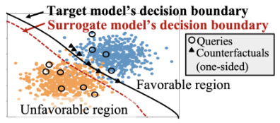
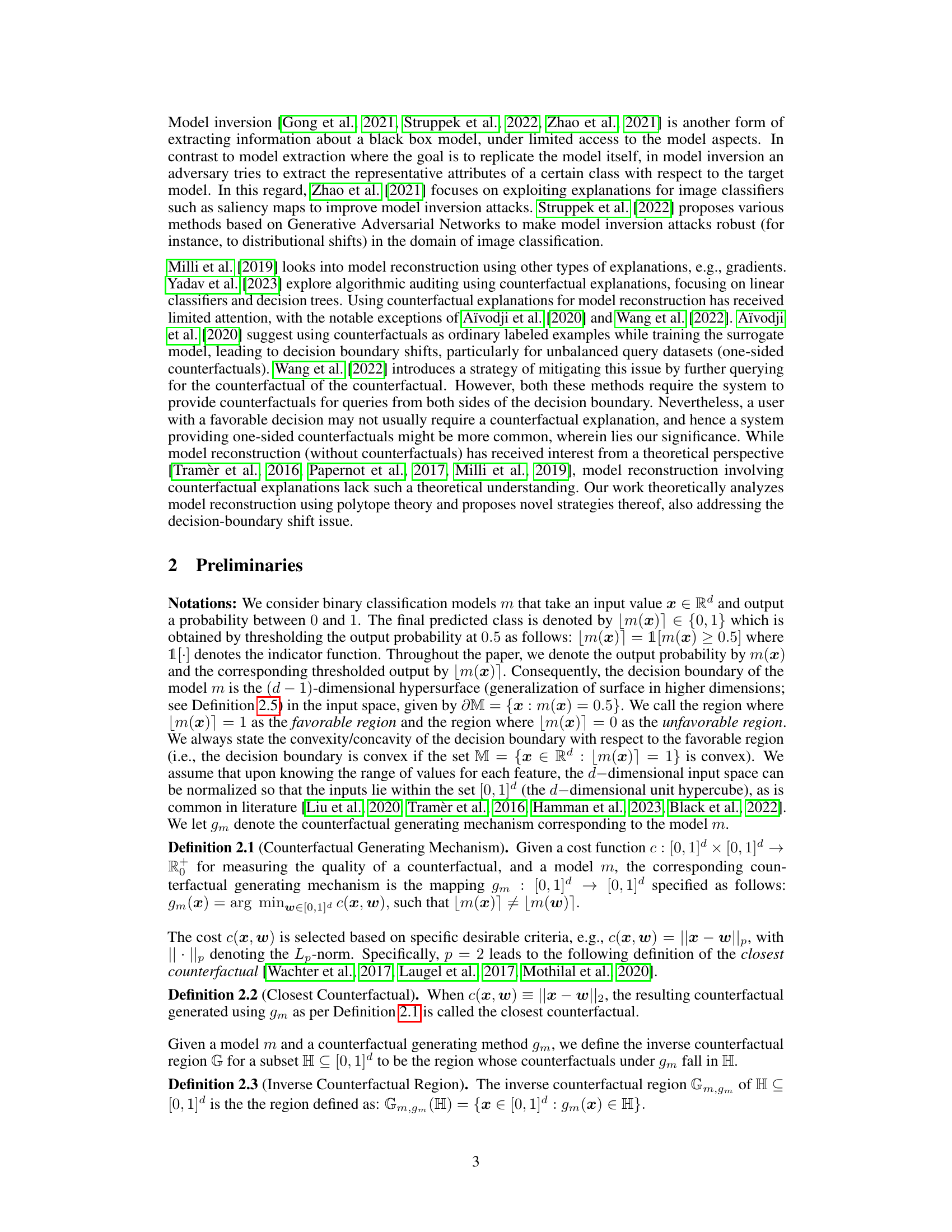
🔼 This figure illustrates the problem of decision boundary shift in model reconstruction using counterfactuals. The black curve represents the decision boundary of the original target model. When counterfactuals (represented by black triangles) are treated as ordinary labeled points during surrogate model training, the surrogate model’s decision boundary (red dashed line) can shift significantly from the target model’s boundary. This shift is particularly problematic when counterfactuals are one-sided (i.e., only available for instances with unfavorable predictions). The figure shows the shift causing misclassifications near the decision boundary.
read the caption
Figure 1: Decision boundary shift when counterfactuals are treated as ordinary labeled points.
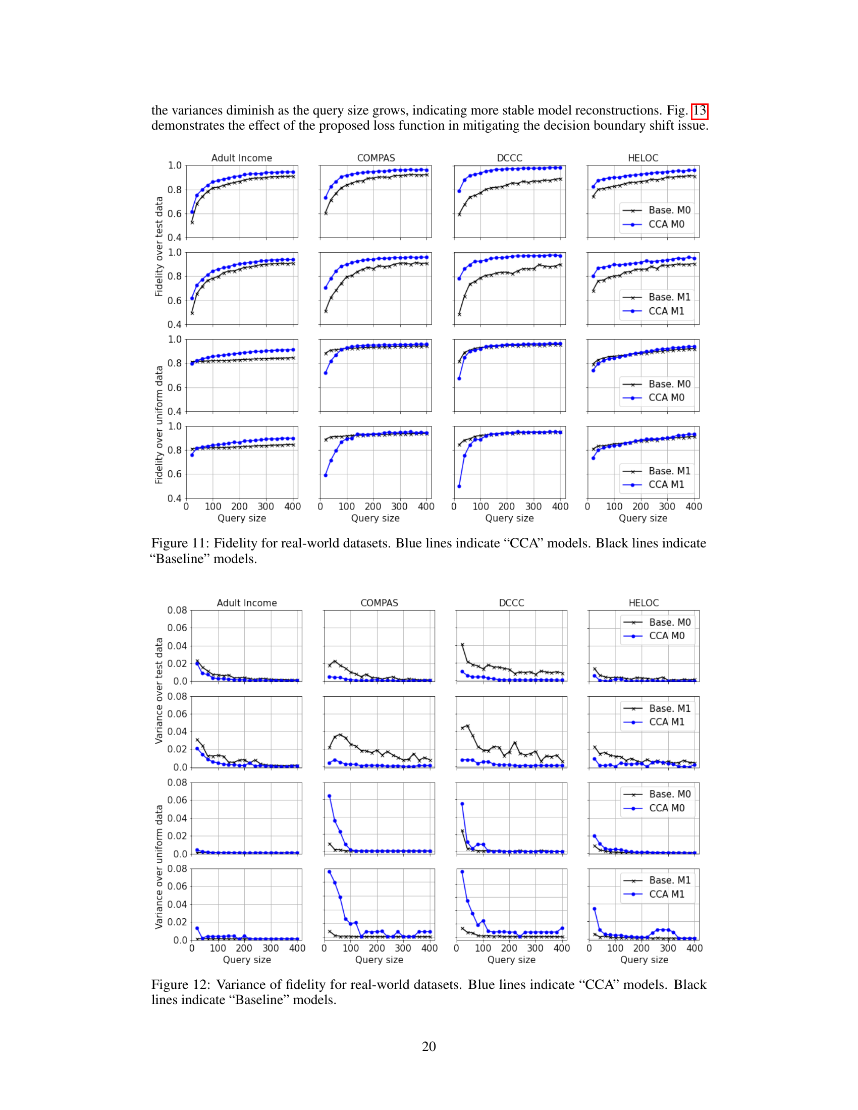
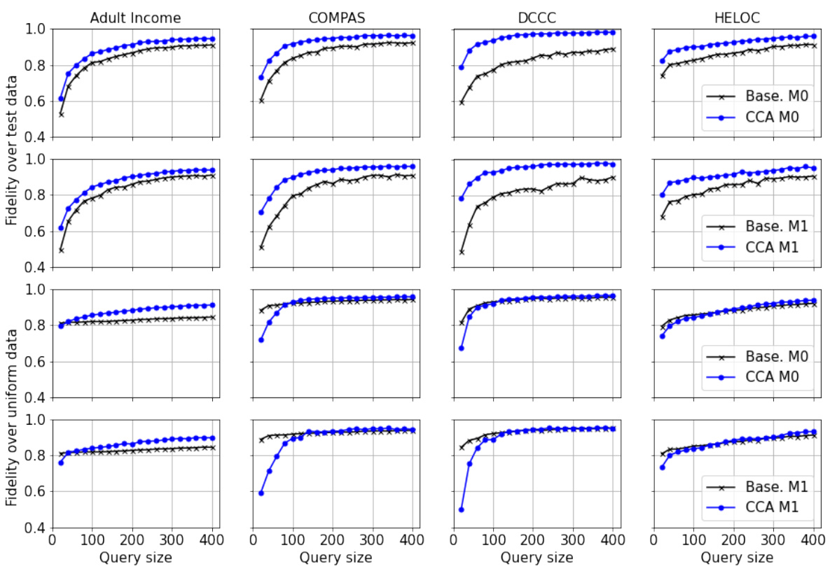
🔼 This table presents the average fidelity results obtained using 400 queries on four real-world datasets (Adult Income, COMPAS, DCCC, and HELOC). The fidelity is calculated for two different surrogate model architectures (Model 0: similar to the target model, Model 1: slightly different). Results are averaged over 100 ensembles, showing the performance of the Counterfactual Clamping Attack (CCA) compared to a baseline method. The table showcases fidelity scores for both uniformly generated data and the test datasets, providing a comprehensive comparison of CCA’s effectiveness in model reconstruction.
read the caption
Table 1: Average fidelity achieved with 400 queries on the real-world datasets over an ensemble of size 100. Target model has hidden layers with neurons (20,10). Model 0 is similar to the target model in architecture. Model 1 has hidden layers with neurons (20, 10, 5).
In-depth insights#
Polytope Theory’s Role#
The research leverages polytope theory to offer rigorous theoretical guarantees on the accuracy of model reconstruction using counterfactual explanations. This is a significant advancement as it moves beyond existing heuristic approaches to provide a deeper understanding of the relationship between the number of counterfactual queries and the resulting reconstruction error. Specifically, the theory is used to analyze scenarios with convex decision boundaries, leading to precise error bounds, and then extended to more complex scenarios involving ReLU networks and locally Lipschitz continuous models, for which probabilistic guarantees are established. The theoretical results directly inform the design of a novel model reconstruction strategy, showcasing the practical utility of this theoretical framework. In essence, polytope theory provides the mathematical foundation for understanding and improving the effectiveness of counterfactual-based model reconstruction attacks.
CCA: A Novel Approach#
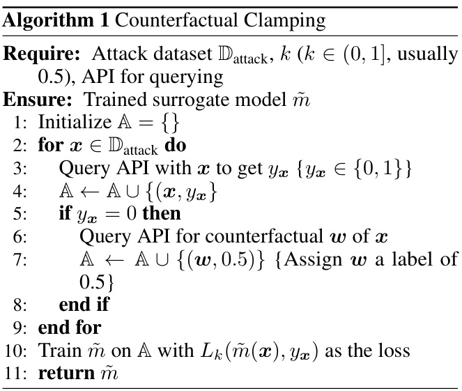
The proposed Counterfactual Clamping Attack (CCA) offers a novel approach to model reconstruction by leveraging the proximity of counterfactuals to the decision boundary. Unlike existing methods, CCA doesn’t treat counterfactuals as standard data points. Instead, it uses a unique loss function that incorporates knowledge about counterfactual location, thereby mitigating the decision boundary shift often observed in other model reconstruction techniques. This strategic handling of counterfactuals leads to improved fidelity between the target and surrogate model predictions. The core innovation lies in its loss function, which differentially penalizes misclassifications depending on whether the instance is a regular data point or a counterfactual. This allows CCA to more accurately learn the decision boundary, even when provided with only one-sided counterfactuals, presenting a significant advantage over existing techniques that demand counterfactuals from both sides of the boundary. The theoretical underpinnings and empirical results support CCA’s efficacy in reconstructing models accurately and efficiently, making it a promising advancement in the field.
One-Sided CF Analysis#
Analyzing counterfactual explanations (CFs) from a one-sided perspective offers valuable insights into model behavior and vulnerabilities. A one-sided approach, where CFs are only generated for instances with unfavorable model predictions, is more realistic in many applications than assuming access to two-sided CFs. This asymmetry introduces new challenges, such as potential decision boundary shift, that must be carefully considered. Theoretical analysis of one-sided CFs, particularly through polytope theory, can provide fundamental guarantees on model reconstruction accuracy and query complexity, revealing the inherent trade-offs between accuracy and the number of queries. Developing model reconstruction strategies that robustly handle one-sided data, such as the Counterfactual Clamping Attack (CCA) mentioned in the paper, is crucial. Furthermore, investigating the relationship between model properties, such as Lipschitz continuity, and the effectiveness of one-sided CF analysis opens avenues for improving model robustness and understanding the limitations of CF-based attacks.
Lipschitz Continuity’s Impact#
The concept of Lipschitz continuity, crucial in analyzing model robustness and generalization, significantly impacts the model reconstruction process using counterfactuals. Models with smaller Lipschitz constants, indicating smoother decision boundaries, are easier to reconstruct because small changes in input lead to proportionally small changes in output. Conversely, models with large Lipschitz constants are more resistant to reconstruction as their decision boundary is highly irregular and thus, require more counterfactual queries for accurate approximation. This is because a high Lipschitz constant suggests that even small perturbations can drastically alter the model’s prediction, and the effectiveness of reconstruction is determined by how closely the surrogate model imitates this behavior near the decision boundary. Therefore, Lipschitz continuity acts as a critical factor influencing the query complexity and fidelity of model reconstruction.
Future Research#
Future research directions stemming from this work on model reconstruction using counterfactual explanations could explore several promising avenues. Extending the theoretical analysis beyond convex and ReLU network assumptions to encompass a broader class of models, including non-convex decision boundaries, is crucial. Investigating the impact of different counterfactual generation methods and their inherent biases on reconstruction accuracy would provide valuable insights. The study could be extended to multi-class classification scenarios to further enhance the model’s practical applicability. Moreover, developing more robust strategies to address the decision boundary shift problem, especially in cases with limited or unbalanced data, is important. Finally, exploring the intersection between model reconstruction attacks and existing defense mechanisms should enhance the security of machine learning systems against these attacks.
More visual insights#
More on figures

🔼 The figure illustrates the model reconstruction problem setting. A target machine learning model is hosted on a Machine Learning as a Service (MLaaS) platform, accessible through an API. An adversary (user) can query the model with a set of input instances (D). The model returns the predictions for these instances and, for the instances with unfavorable predictions, provides corresponding counterfactuals. The adversary aims to build a surrogate model that closely mimics the target model based on these queries and counterfactuals. This setup highlights the interplay between model explainability and privacy.
read the caption
Figure 2: Problem setting

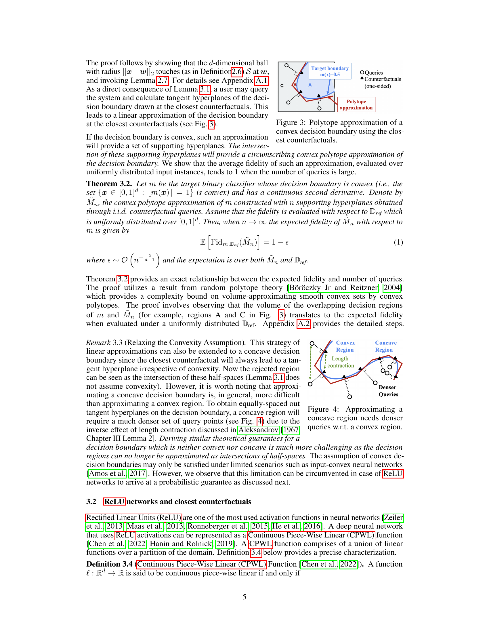
🔼 This figure illustrates how a convex decision boundary can be approximated using a polytope constructed from supporting hyperplanes obtained through counterfactual queries. The target model’s decision boundary (a curve) is approximated by a polygon formed by the intersections of tangent hyperplanes at each of the closest counterfactuals. The figure highlights the queries, the resulting counterfactuals (one-sided), and the resulting polytope approximation.
read the caption
Figure 3: Polytope approximation of a convex decision boundary using the closest counterfactuals.
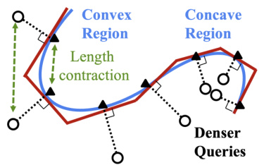
🔼 This figure illustrates the difference in query density required for approximating convex versus concave decision boundaries. In a convex region, the tangent hyperplanes obtained from closest counterfactuals are relatively well-spaced. However, in a concave region, due to length contraction, a much denser set of query points is needed to obtain equally spaced tangent hyperplanes that provide an accurate approximation of the decision boundary.
read the caption
Figure 4: Approximating a concave region needs denser queries w.r.t. a convex region.

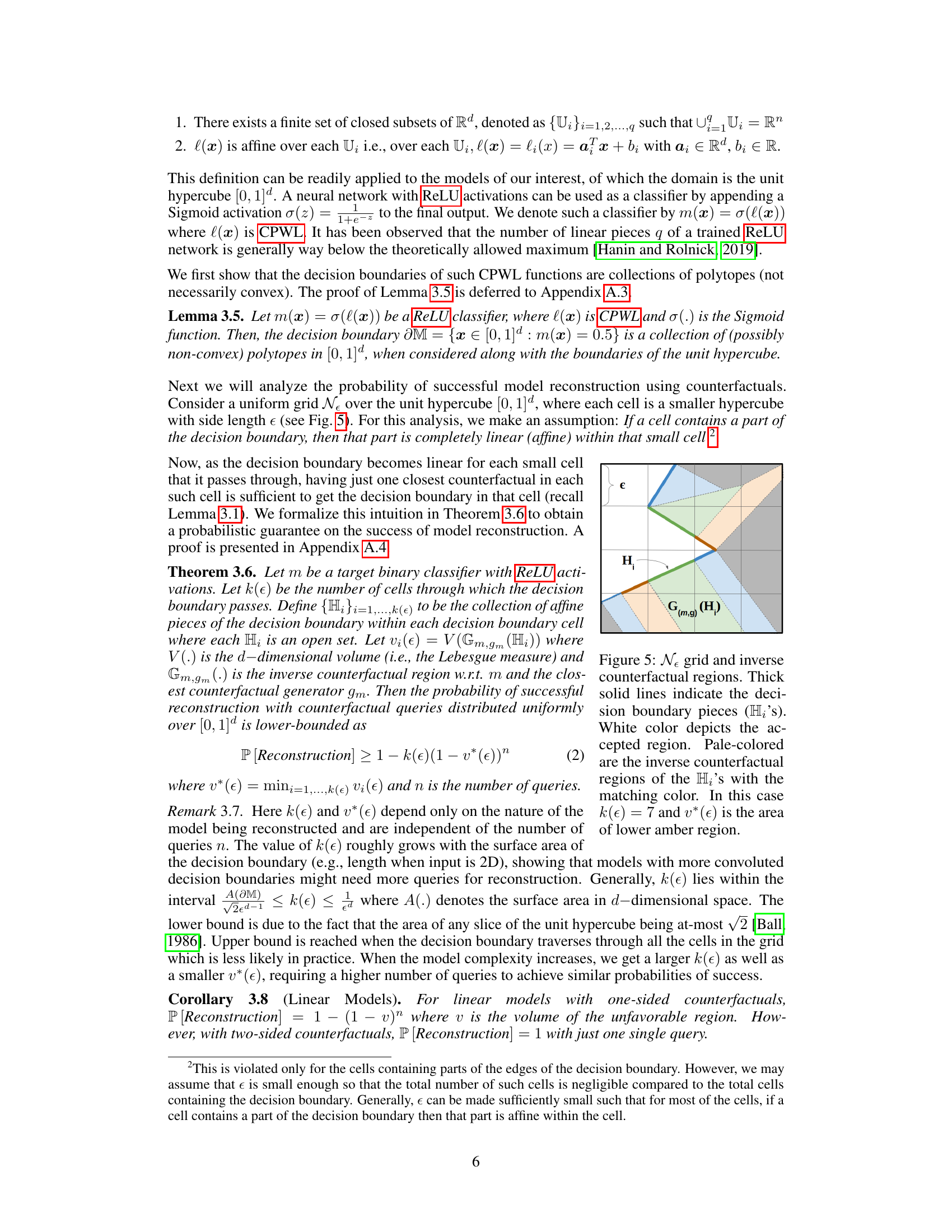
🔼 This figure illustrates the concept of inverse counterfactual regions within a uniform grid. The decision boundary is broken into linear pieces within each cell. The inverse counterfactual region for a piece of the decision boundary (Hi) is the set of points whose closest counterfactuals fall within Hi. The figure visually demonstrates how the volume of these inverse counterfactual regions (vi(e)) influences the probability of successful model reconstruction. The area of the lower amber region represents the minimum volume (v*(e)) across all regions.
read the caption
Figure 5: Ne grid and inverse counterfactual regions. Thick solid lines indicate the decision boundary pieces (Hi's). White color depicts the accepted region. Pale-colored are the inverse counterfactual regions of the Hi's with the matching color. In this case k(e) = 7 and v*(e) is the area of lower amber region.

🔼 This figure illustrates the core idea behind the Counterfactual Clamping Attack (CCA). The target model’s decision boundary (red curve) and surrogate model’s decision boundary (blue curve) are shown. The green circles represent the counterfactuals, which lie near the decision boundary. The goal is to force the surrogate model to make similar predictions to the target model around these counterfactuals by using a unique loss function. The dotted lines connect the counterfactuals to their corresponding instances. The loss function penalizes the surrogate model only if its prediction is lower than a threshold for the counterfactuals, ensuring that the surrogate model’s decision boundary remains close to that of the target model for counterfactuals.
read the caption
Figure 6: Rationale for Counterfactual Clamping Strategy.

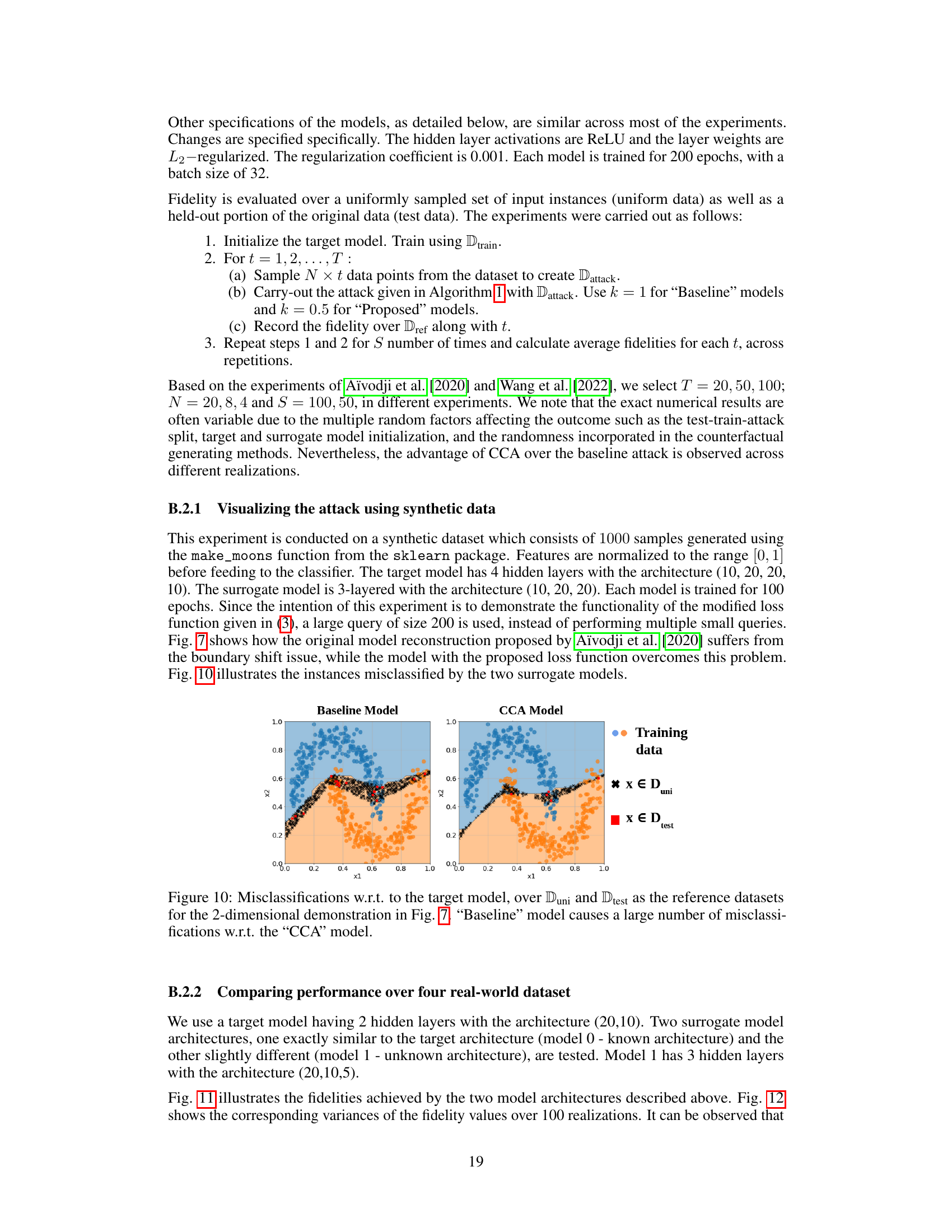
🔼 This figure provides a visual comparison of three different models on a 2D synthetic dataset: the target model, the baseline model (from Aïvodji et al., 2020), and the CCA model (the authors’ proposed method). It illustrates how the baseline model suffers from decision boundary shift, while the CCA model effectively mitigates this issue, resulting in a more accurate approximation of the target model’s decision boundary. The colors represent the predicted class for each region (orange for one class, blue for the other), and the different symbols show the types of data points used: training data, counterfactuals, and queries. The figure demonstrates the efficacy of the CCA model in reconstructing the target model’s decision boundary by using a modified loss function that addresses the issue of decision boundary shifts.
read the caption
Figure 7: A 2-D demonstration of the proposed strategy. Orange and blue shades denote the favorable and unfavorable decision regions of each model. Circles denote the target model's training data.
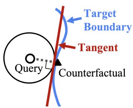
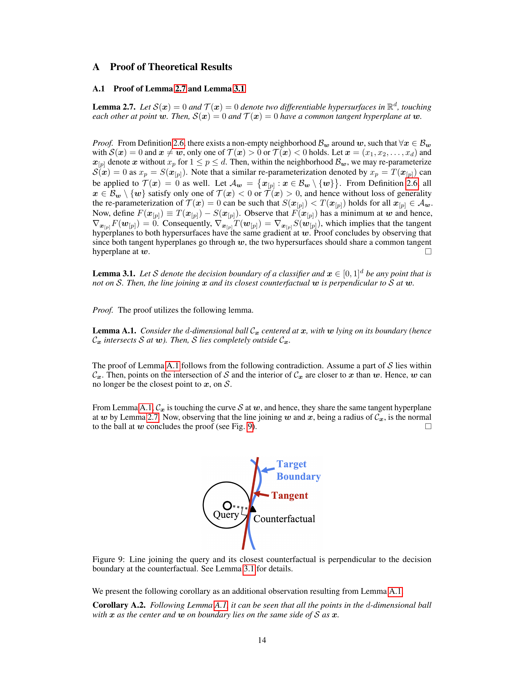
🔼 The figure shows a geometrical illustration of Lemma 3.1. A query point is shown with its closest counterfactual on a decision boundary. A line connecting the query and counterfactual is shown perpendicular to the tangent of the decision boundary at the point of the counterfactual. This illustrates that the line connecting a query point and its closest counterfactual is perpendicular to the decision boundary at the counterfactual point.
read the caption
Figure 9: Line joining the query and its closest counterfactual is perpendicular to the decision boundary at the counterfactual. See Lemma 3.1 for details.

🔼 This figure compares the decision boundaries of three models: the target model, a baseline model, and the CCA model. The orange and blue regions represent the positive and negative classes, respectively, for each model. The target model’s training data points are shown as circles. The plot shows how the baseline model suffers from decision boundary shift, while CCA model produces a decision boundary that is more aligned with the target model, indicating improved model reconstruction.
read the caption
Figure 7: A 2-D demonstration of the proposed strategy. Orange and blue shades denote the favorable and unfavorable decision regions of each model. Circles denote the target model’s training data.
🔼 This figure compares the decision boundaries of three models in a two-dimensional space: the target model, a baseline model trained with a standard loss function, and a CCA (Counterfactual Clamping Attack) model trained with the proposed loss function. The different colored regions represent the favorable and unfavorable regions of each model. The plot illustrates how the CCA model better approximates the decision boundary of the target model compared to the baseline model, which demonstrates the effectiveness of CCA in mitigating decision boundary shift.
read the caption
Figure 7: A 2-D demonstration of the proposed strategy. Orange and blue shades denote the favorable and unfavorable decision regions of each model. Circles denote the target model’s training data.

🔼 This figure shows a 2D visualization comparing the target model’s decision boundary with those of the baseline model and the CCA model. The orange and blue shades represent the favorable and unfavorable regions for each model. Circles indicate the training data points from the original target model. The figure visually demonstrates how the CCA model’s decision boundary is much closer to the target model’s boundary, in contrast to the baseline model, which exhibits a larger decision boundary shift.
read the caption
Figure 7: A 2-D demonstration of the proposed strategy. Orange and blue shades denote the favorable and unfavorable decision regions of each model. Circles denote the target model’s training data.

🔼 This figure visualizes the performance of the proposed Counterfactual Clamping Attack (CCA) method compared to a baseline method on a synthetic 2D dataset. The orange and blue regions represent the favorable and unfavorable prediction regions, respectively, for each model. The plot shows that the baseline model’s decision boundary shifts away from the true boundary, indicating a problem with existing methods. In contrast, CCA’s decision boundary better approximates the true boundary, illustrating its effectiveness.
read the caption
Figure 7: A 2-D demonstration of the proposed strategy. Orange and blue shades denote the favorable and unfavorable decision regions of each model. Circles denote the target model's training data.
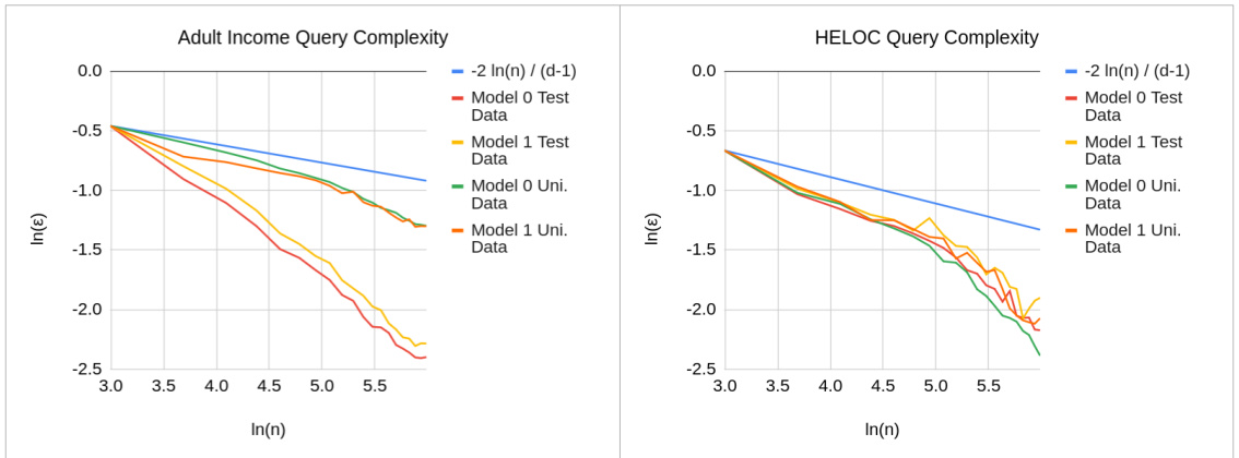
🔼 This figure compares the theoretical query complexity from Theorem 3.2 with empirical results from Adult Income and HELOC datasets. The log-log scale graphs show that the theoretical complexity provides an upper bound for the empirical complexities found in the experiments. Note that a constant was added to the graphs for presentation purposes, which does not change the slope of the lines representing the complexities.
read the caption
Figure 14: A comparison of the query complexity derived in Theorem 3.2 with the empirical query complexities obtained on the Adult Income and HELOC datasets. The graphs are on a log-log scale. We observe that the analytical query complexity is an upper bound for the empirical query complexities. All the graphs are recentered with an additive constant for presentational convenience. However, this does not affect the slope of the graph, which corresponds to the complexity.

🔼 This figure visually demonstrates the effectiveness of the proposed counterfactual clamping (CCA) strategy compared to a baseline method. A synthetic 2D dataset is used to illustrate how CCA mitigates decision boundary shift. The orange and blue regions represent the favorable and unfavorable regions predicted by each model (target, baseline, and CCA). The circles represent the training data points used to train the target model. The figure clearly shows that the CCA model’s decision boundary (blue/orange separation) is a much closer approximation to the target model’s decision boundary than the baseline model’s decision boundary. This highlights the CCA strategy’s improved fidelity in reconstructing the target model’s behavior.
read the caption
Figure 7: A 2-D demonstration of the proposed strategy. Orange and blue shades denote the favorable and unfavorable decision regions of each model. Circles denote the target model's training data.

🔼 This figure shows a 2D visualization comparing the target model, the baseline model (without counterfactual clamping), and the CCA model (with counterfactual clamping). The orange and blue regions represent the favorable and unfavorable prediction regions of each model. The plots illustrate how the baseline model suffers from decision boundary shift while CCA improves model reconstruction fidelity by better aligning the surrogate model’s decision boundary with that of the target model.
read the caption
Figure 7: A 2-D demonstration of the proposed strategy. Orange and blue shades denote the favorable and unfavorable decision regions of each model. Circles denote the target model's training data.
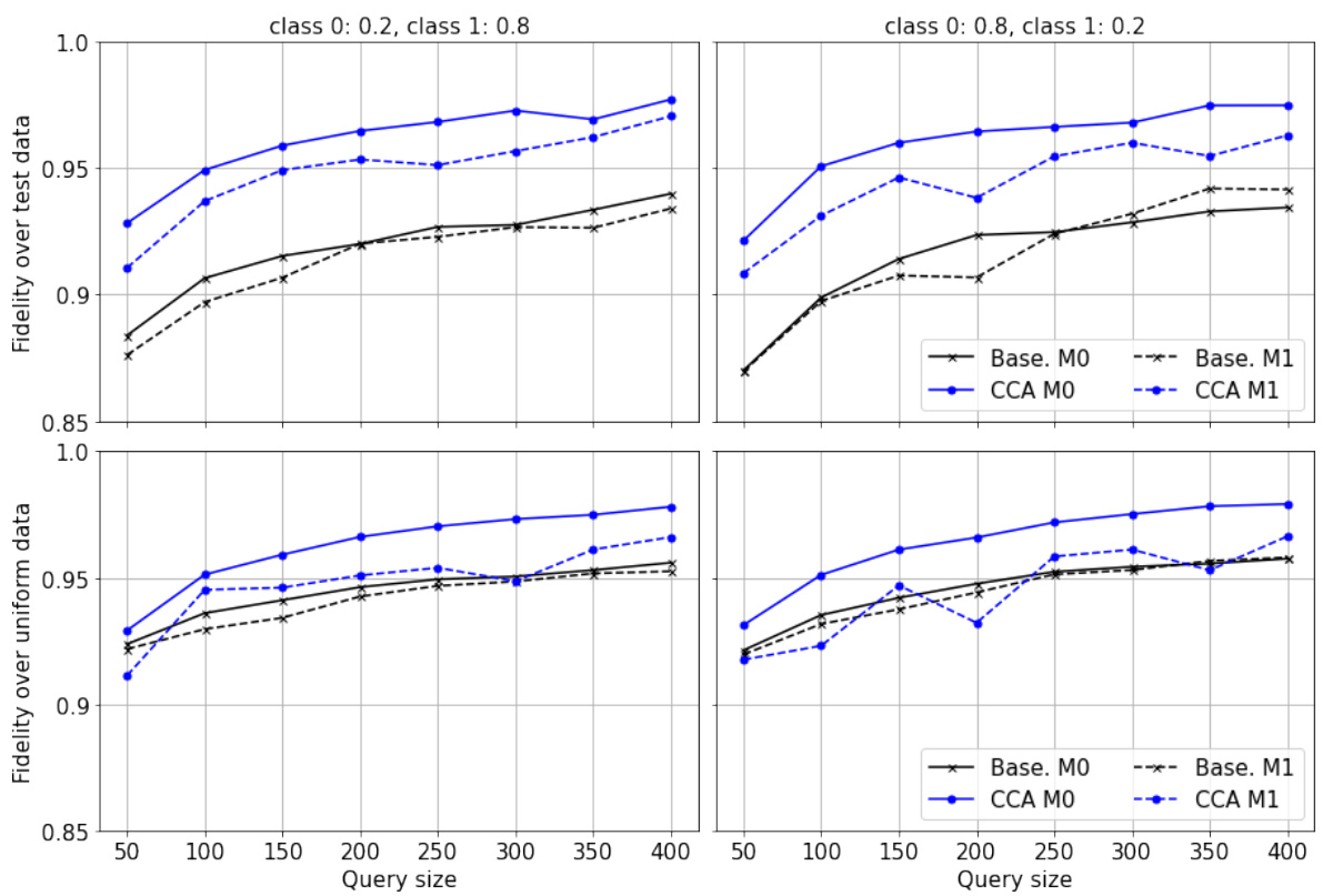
🔼 This figure visualizes the performance of the proposed Counterfactual Clamping Attack (CCA) strategy compared to a baseline method on a 2D synthetic dataset. The orange and blue regions represent the favorable and unfavorable prediction areas, respectively. The circles indicate the target model’s training data. The figure demonstrates that CCA effectively mitigates decision boundary shift, a common problem in model reconstruction approaches that use counterfactuals as ordinary data points. In contrast to the baseline method, CCA produces a surrogate model with a decision boundary that closely aligns with the target model.
read the caption
Figure 7: A 2-D demonstration of the proposed strategy. Orange and blue shades denote the favorable and unfavorable decision regions of each model. Circles denote the target model's training data.
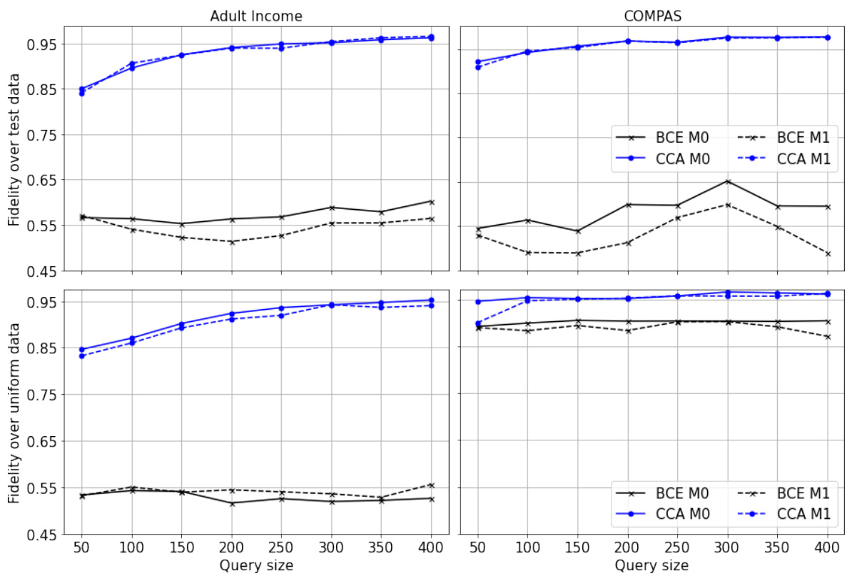
🔼 This figure compares the probability distributions of predictions made by the baseline model and the CCA model for the HELOC dataset. It highlights how CCA mitigates the decision boundary shift, resulting in a distribution where counterfactuals are clustered around 0.5, and other instances are around 1.0.
read the caption
Figure 13: Histograms of probabilities predicted by “Baseline” and “CCA” models under the “Unknown Architecture” scenario (model 1) for the HELOC dataset. Note how the “Baseline” model provides predictions higher than 0.5 for a comparatively larger number of instances with [m(x)] = 0 due to the boundary shift issue. The clamping effect of the novel loss function is evident in the “CCA” model’s histogram, where the decision boundary being held closer to the counterfactuals is causing the two prominent modes in the favorable region. The mode closer to 0.5 is due to counterfactuals and the mode closer to 1.0 is due to instances with [m(x)] = 1.
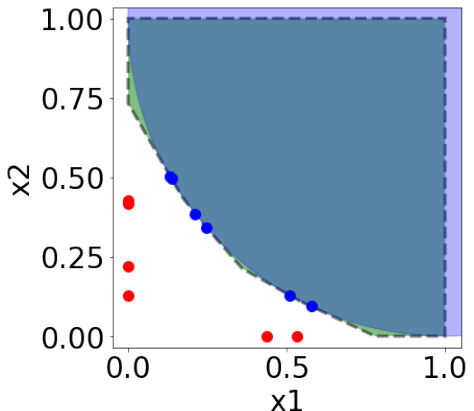
🔼 This figure illustrates how a convex decision boundary can be approximated using a polytope. The target model’s decision boundary (a curve) is shown in dark blue. Red dots represent one-sided counterfactual queries (points for which the model prediction was unfavorable). Blue dots represent the corresponding closest counterfactuals (points that yield a favorable outcome with minimum perturbation). The dashed black line shows the polytope approximation of the decision boundary which is created by the intersection of the tangent hyperplanes at each counterfactual point. The shaded green region highlights the area where the approximation differs from the target model’s decision boundary.
read the caption
Figure 3: Polytope approximation of a convex decision boundary using the closest counterfactuals.
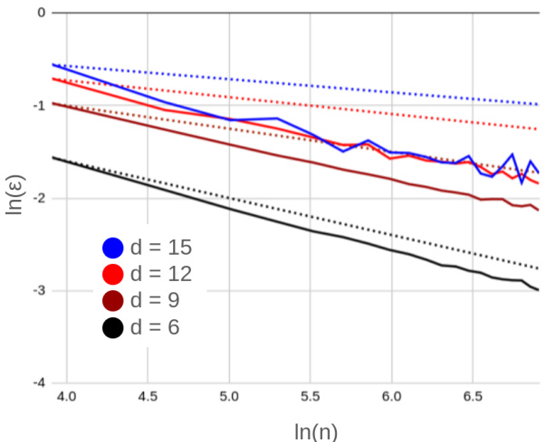
🔼 This figure validates Theorem 3.2 by comparing the theoretical and empirical rates of convergence of the approximation error (epsilon) with the number of queries (n) for different dimensionality values (d). The dotted lines represent the theoretical rates, and the solid lines represent the empirical results obtained from experiments. The plot uses logarithmic scales for both epsilon and n, allowing for better visualization of the convergence behavior. The results show that the empirical convergence rates generally follow the predicted theoretical rates, with some deviation observed at higher dimensions.
read the caption
Figure 20: Verifying Theorem 3.2: Dotted and solid lines indicate the theoretical and empirical rates of convergence.
More on tables

🔼 This table presents the average fidelity achieved by the Counterfactual Clamping Attack (CCA) and the baseline method for four real-world datasets. The fidelity is calculated using two different reference datasets: uniformly distributed samples (Duni) and test dataset samples (Dtest). Two surrogate model architectures are compared: one similar to the target model (Model 0) and one with a different architecture (Model 1). The results show the fidelity values for each method, dataset, and reference dataset.
read the caption
Table 1: Average fidelity achieved with 400 queries on the real-world datasets over an ensemble of size 100. Target model has hidden layers with neurons (20,10). Model 0 is similar to the target model in architecture. Model 1 has hidden layers with neurons (20, 10, 5).
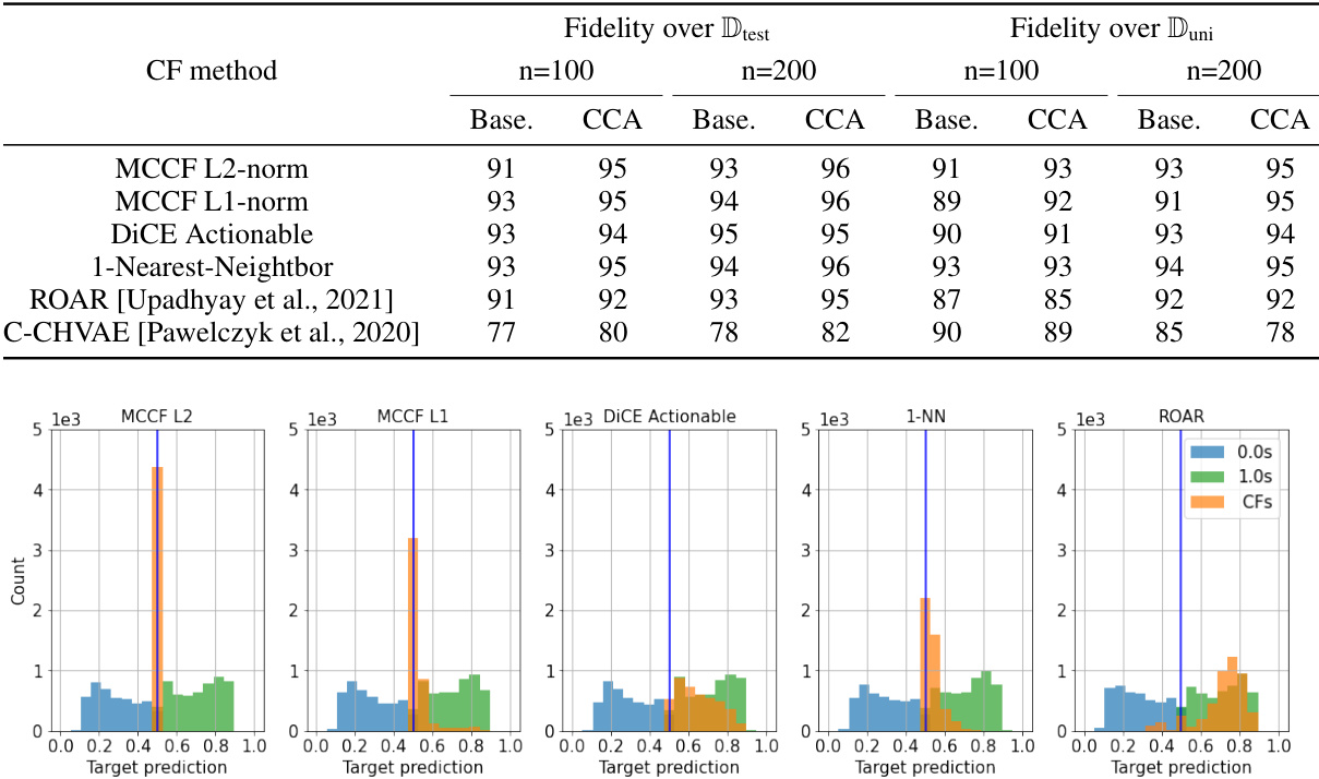
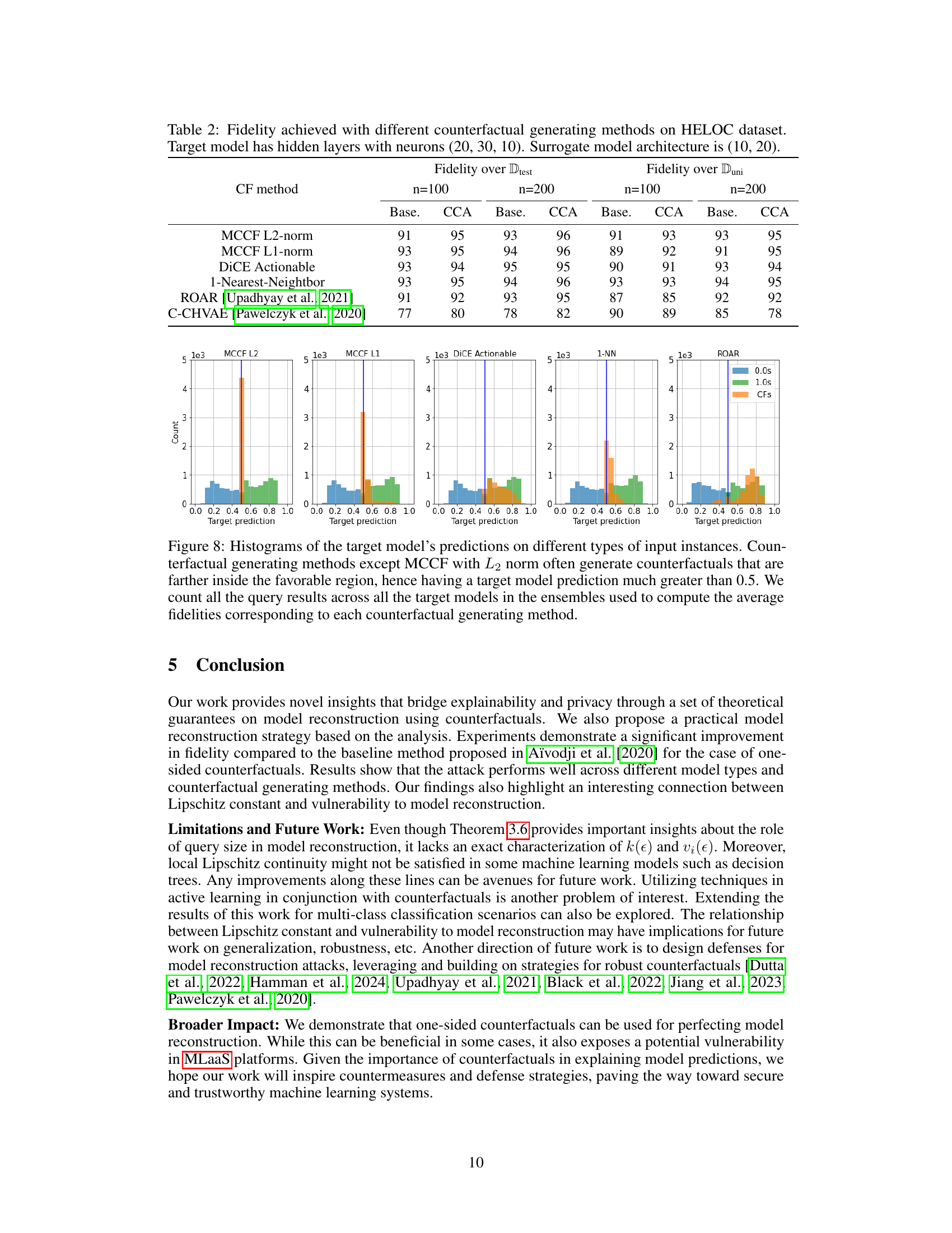
🔼 This table presents the fidelity results achieved using different counterfactual generation methods on the HELOC dataset. The target model has three hidden layers with (20, 30, 10) neurons while the surrogate model has two hidden layers with (10, 20) neurons. It compares the performance of the proposed Counterfactual Clamping Attack (CCA) with a baseline approach using different counterfactual generation techniques, including MCCF with L2 and L1 norms, DiCE Actionable, 1-Nearest-Neighbor, ROAR, and C-CHVAE. Fidelity is measured for different query sizes (n=100 and n=200). The table also includes histograms visualizing the distribution of target model predictions for each counterfactual generation method.
read the caption
Table 2: Fidelity achieved with different counterfactual generating methods on HELOC dataset. Target model has hidden layers with neurons (20, 30, 10). Surrogate model architecture is (10, 20).

🔼 This table presents the average fidelity results obtained by using 400 queries on four real-world datasets. Two different surrogate model architectures are tested: one similar and one slightly different from the target model’s architecture. The fidelity is measured for both uniformly sampled instances and test data instances. The table shows that the proposed CCA method generally achieves higher or similar fidelity compared to the baseline method.
read the caption
Table 1: Average fidelity achieved with 400 queries on the real-world datasets over an ensemble of size 100. Target model has hidden layers with neurons (20,10). Model 0 is similar to the target model in architecture. Model 1 has hidden layers with neurons (20, 10, 5).
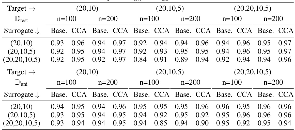
🔼 This table shows the average fidelity achieved by using the proposed Counterfactual Clamping Attack (CCA) and the baseline method on four real-world datasets. The results are presented for two different surrogate model architectures, one similar to the target model and one with a different number of layers. The fidelity is measured using two different reference datasets: one with uniformly distributed samples and one with test data instances.
read the caption
Table 1: Average fidelity achieved with 400 queries on the real-world datasets over an ensemble of size 100. Target model has hidden layers with neurons (20,10). Model 0 is similar to the target model in architecture. Model 1 has hidden layers with neurons (20, 10, 5).
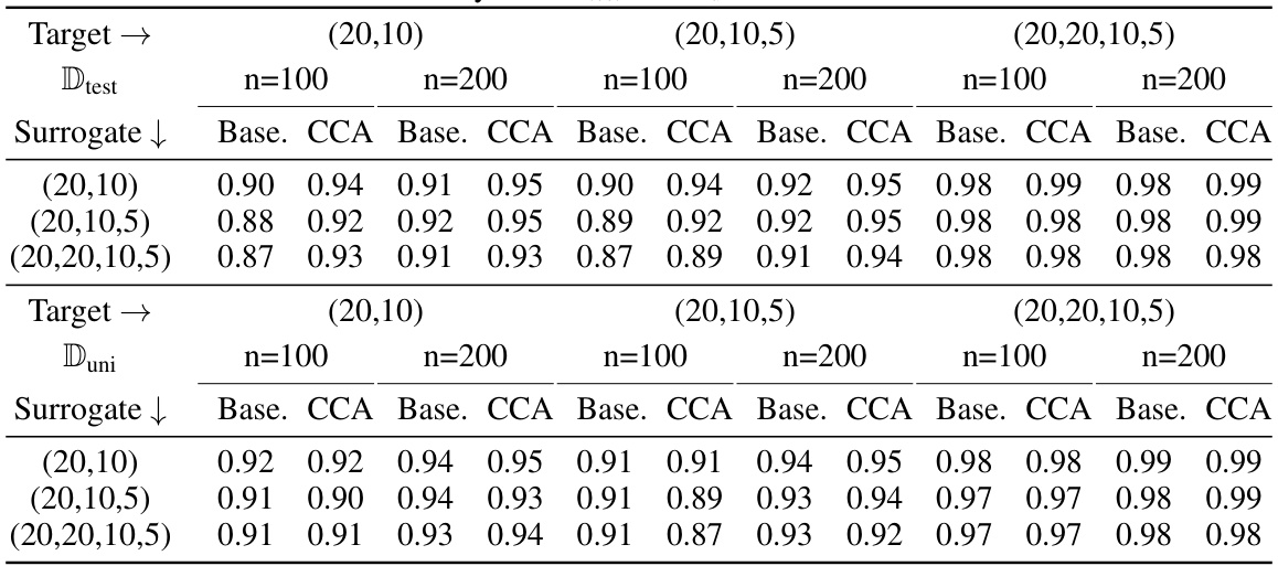
🔼 This table presents the average fidelity results achieved by using 400 queries on four real-world datasets. The fidelity is measured using two different surrogate models (Model 0 and Model 1) with varying architectures. Two different methods are compared for model reconstruction: the baseline method and the proposed CCA method. The results are presented for two different reference datasets: one with uniformly generated data points and one using the actual test data. The table shows how the proposed method improves fidelity of reconstruction compared to the baseline method across different datasets and model architectures.
read the caption
Table 1: Average fidelity achieved with 400 queries on the real-world datasets over an ensemble of size 100. Target model has hidden layers with neurons (20,10). Model 0 is similar to the target model in architecture. Model 1 has hidden layers with neurons (20, 10, 5).

🔼 This table presents the average fidelity achieved by using the Counterfactual Clamping Attack (CCA) and the baseline method on four real-world datasets. Two different surrogate model architectures were tested (Model 0, similar to the target model, and Model 1, with a different architecture) for each dataset. The fidelity was calculated using 400 queries on an ensemble of 100 target models.
read the caption
Table 1: Average fidelity achieved with 400 queries on the real-world datasets over an ensemble of size 100. Target model has hidden layers with neurons (20,10). Model 0 is similar to the target model in architecture. Model 1 has hidden layers with neurons (20, 10, 5).
Full paper#
