TL;DR#
Traditional diffusion models for image generation require many steps, making them computationally expensive and producing latent spaces that are not easily interpretable. This slow process limits applications like video generation and editing. Additionally, many existing models struggle with achieving high-quality image generation with only a single denoising step, hampering efficiency.
The proposed UDPM model addresses these limitations by integrating downsampling and upsampling into the diffusion process. This approach drastically reduces the computational cost, generating high-quality images with significantly fewer steps. UDPM’s superior performance, demonstrated on various image datasets, and interpretable latent space provide a significant advancement. Its innovative approach provides a promising new avenue for efficient and versatile image generation.
Key Takeaways#
Why does it matter?#
This paper is important because it presents UDPM, a novel approach to image generation that significantly improves efficiency and interpretability. Its faster sampling and improved latent space make it highly relevant to current research in generative models, and it could open new avenues in areas such as image editing and manipulation.
Visual Insights#

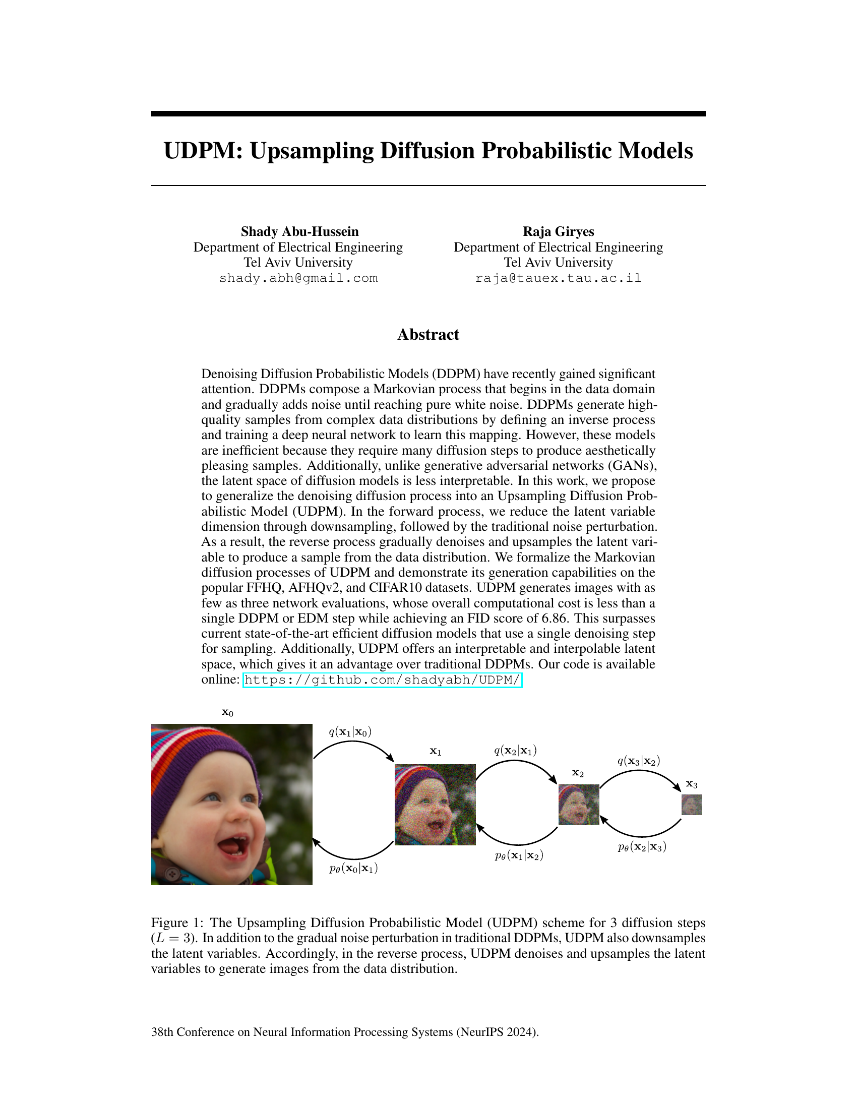
🔼 This figure illustrates the process of the Upsampling Diffusion Probabilistic Model (UDPM). It shows how UDPM differs from traditional Denoising Diffusion Probabilistic Models (DDPMs) by incorporating downsampling steps in the forward diffusion process (adding noise and reducing resolution) and corresponding upsampling steps in the reverse diffusion process (denoising and increasing resolution). The forward process starts with an image (X0) and gradually adds noise while downsampling the image until pure noise (X3) is achieved. The reverse process learns to denoise and upsample the latent variables, eventually reconstructing the original image.
read the caption
Figure 1: The Upsampling Diffusion Probabilistic Model (UDPM) scheme for 3 diffusion steps (L = 3). In addition to the gradual noise perturbation in traditional DDPMs, UDPM also downsamples the latent variables. Accordingly, in the reverse process, UDPM denoises and upsamples the latent variables to generate images from the data distribution.
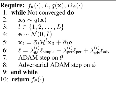
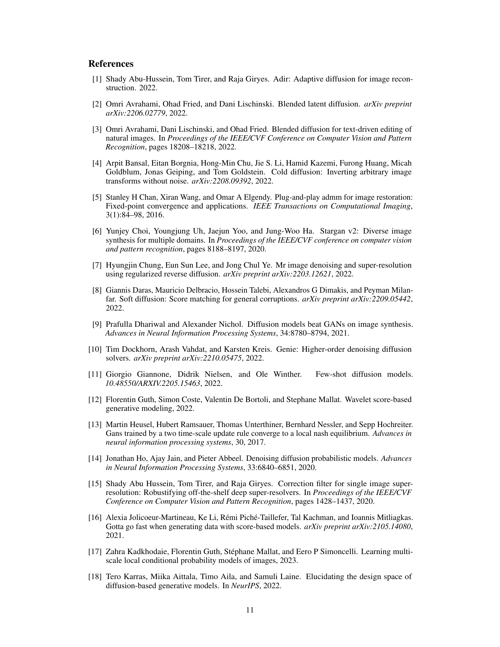
🔼 This table compares the Fréchet Inception Distance (FID) scores of UDPM against other state-of-the-art diffusion models on the CIFAR10 dataset. It highlights UDPM’s efficiency by showing that its 3 steps are computationally equivalent to only 0.3 steps of a typical diffusion model. Lower FID scores indicate better image quality.
read the caption
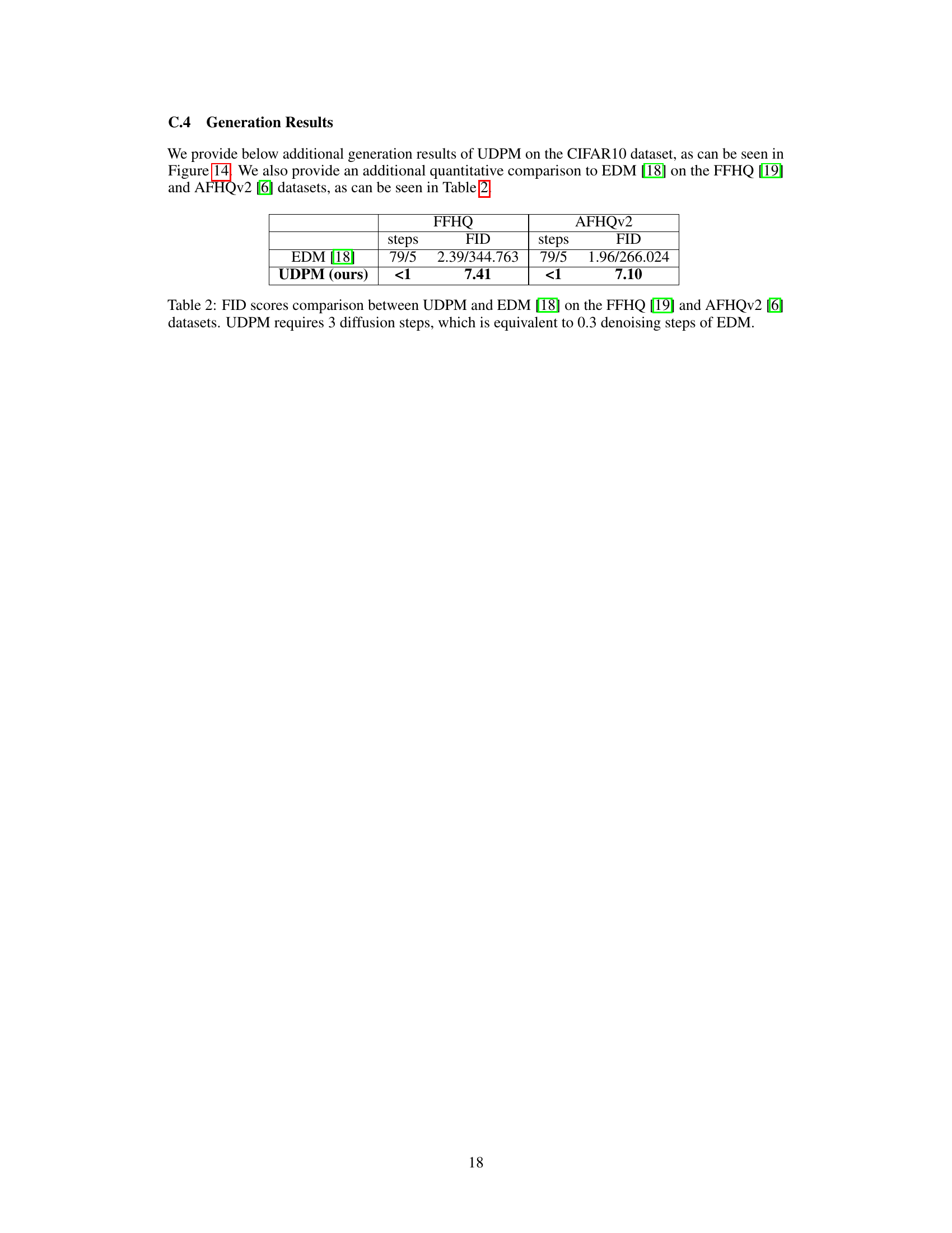
Table 1: FID scores on the CIFAR10 dataset [22]. UDPM uses 3 steps, which are equivalent in terms of complexity to 0.3 of a single denoising step used in typical diffusion models like DDPM or EDM.
In-depth insights#
UDPM: A New Model#
The proposed UDPM model presents a novel approach to diffusion probabilistic models by integrating downsampling into the forward diffusion process. This key innovation results in a more efficient model, requiring fewer steps to generate high-quality samples compared to traditional DDPMs. Reduced computational cost is a significant advantage, making the model more practical for various applications. Furthermore, the inclusion of downsampling provides an interpretable latent space, allowing for manipulation and interpolation of generated images in a manner similar to GANs. Improved interpretability is a crucial distinction from typical DDPMs, opening new possibilities for image editing and other generative tasks. However, the paper’s evaluation is limited to a few datasets, and further investigation across broader datasets and applications is warranted to fully understand the model’s generalizability and robustness.
Upsampling Diffusion#
Upsampling diffusion presents a novel approach to generative modeling by integrating upsampling operations within the diffusion process. Instead of solely relying on noise addition and removal, this method strategically reduces the dimensionality of the latent space through downsampling before adding noise, making it more computationally efficient. The reverse process, then, involves simultaneous denoising and upsampling, gradually reconstructing the high-resolution image. This technique offers several advantages, including reduced computational cost due to working with smaller latent representations during training and inference and potential improved interpretability of the latent space. However, challenges might include the careful design of upsampling operations to avoid artifacts and the need for thorough evaluation on diverse datasets to validate the method’s generalization capabilities. The trade-off between computational savings and the potential introduction of artifacts in the upsampling process is an area that requires further investigation.
Efficient Sampling#
Efficient sampling in diffusion models is crucial for practical applications, as the standard process can be computationally expensive. The core challenge lies in reducing the number of denoising steps required to generate high-quality samples without sacrificing image fidelity. Upsampling Diffusion Probabilistic Models (UDPM), for instance, address this by introducing a downsampling step in the forward diffusion process, thus reducing the dimensionality of the latent variables. This leads to a more efficient reverse process with fewer denoising steps required, resulting in significantly faster sampling. The efficiency gains stem from reduced computational cost per step and fewer steps overall. However, it’s important to note that the efficiency improvements often come with trade-offs. For example, while UDPM offers speed advantages, its latent space might be less interpretable. Therefore, the choice of an efficient sampling method depends on the specific needs of the application, balancing speed with the desired image quality and interpretability of the latent space. Future research should explore even more efficient techniques without sacrificing performance or interpretability.
Interpretable Latent#
The concept of “Interpretable Latent” space in generative models, especially diffusion models, is crucial for enhancing user control and understanding. Traditional diffusion models often suffer from a lack of interpretability in their latent representations, making it difficult to understand how latent variables influence the generated output. An “Interpretable Latent” space would ideally allow for intuitive manipulation of these latent features, enabling targeted modifications to the generated content such as changing attributes or styles. This improved interpretability could facilitate advancements in areas like image editing, style transfer, and conditional generation. By making the latent space more interpretable, users can gain a deeper understanding of the model’s internal representations, leading to better control and creativity in generating new outputs. A key challenge is to design architectures and training procedures that explicitly promote interpretability without sacrificing the model’s generative quality. Methods like incorporating disentangled latent representations or using lower-dimensional latent spaces could potentially address this challenge. Achieving a truly interpretable latent space represents a significant step toward more transparent and controllable generative models.
Future Works#
The paper’s core contribution, the UDPM, presents exciting avenues for future research. Improving efficiency remains a key goal; exploring alternative downsampling and upsampling techniques beyond simple blurring and strided convolutions could yield significant speedups. Furthermore, extending UDPM to handle more complex data modalities like video or 3D point clouds is a natural next step, requiring careful adaptation of the downsampling and noise injection strategies. Investigating the latent space’s potential for image manipulation tasks beyond simple interpolation is crucial, potentially paving the way for advanced editing applications. A thorough exploration of different loss functions and training schemes could further enhance UDPM’s performance. Finally, thorough comparison with state-of-the-art models on larger datasets and a careful analysis of the model’s limitations, particularly concerning generalization and robustness, would solidify UDPM’s position within the diffusion model landscape.
More visual insights#
More on figures

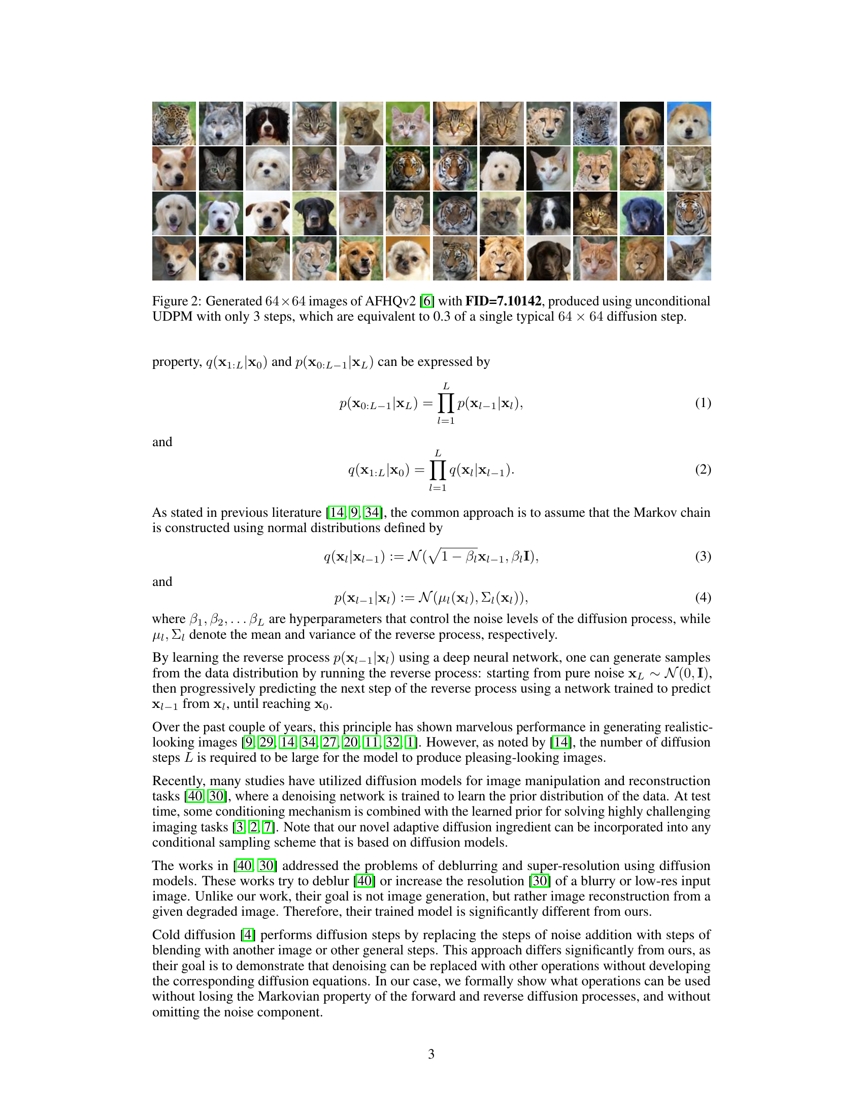
🔼 This figure shows 64x64 images of animals generated using the proposed unconditional Upsampling Diffusion Probabilistic Model (UDPM). The model uses only three diffusion steps to generate these images. The Fréchet Inception Distance (FID) score, a metric for evaluating the quality of generated images, is reported as 7.10142, indicating high fidelity. The caption highlights the efficiency of the UDPM, noting that its three steps are computationally equivalent to only 0.3 of a single step in traditional diffusion models.
read the caption
Figure 2: Generated 64 × 64 images of AFHQv2 [6] with FID=7.10142, produced using unconditional UDPM with only 3 steps, which are equivalent to 0.3 of a single typical 64 × 64 diffusion step.

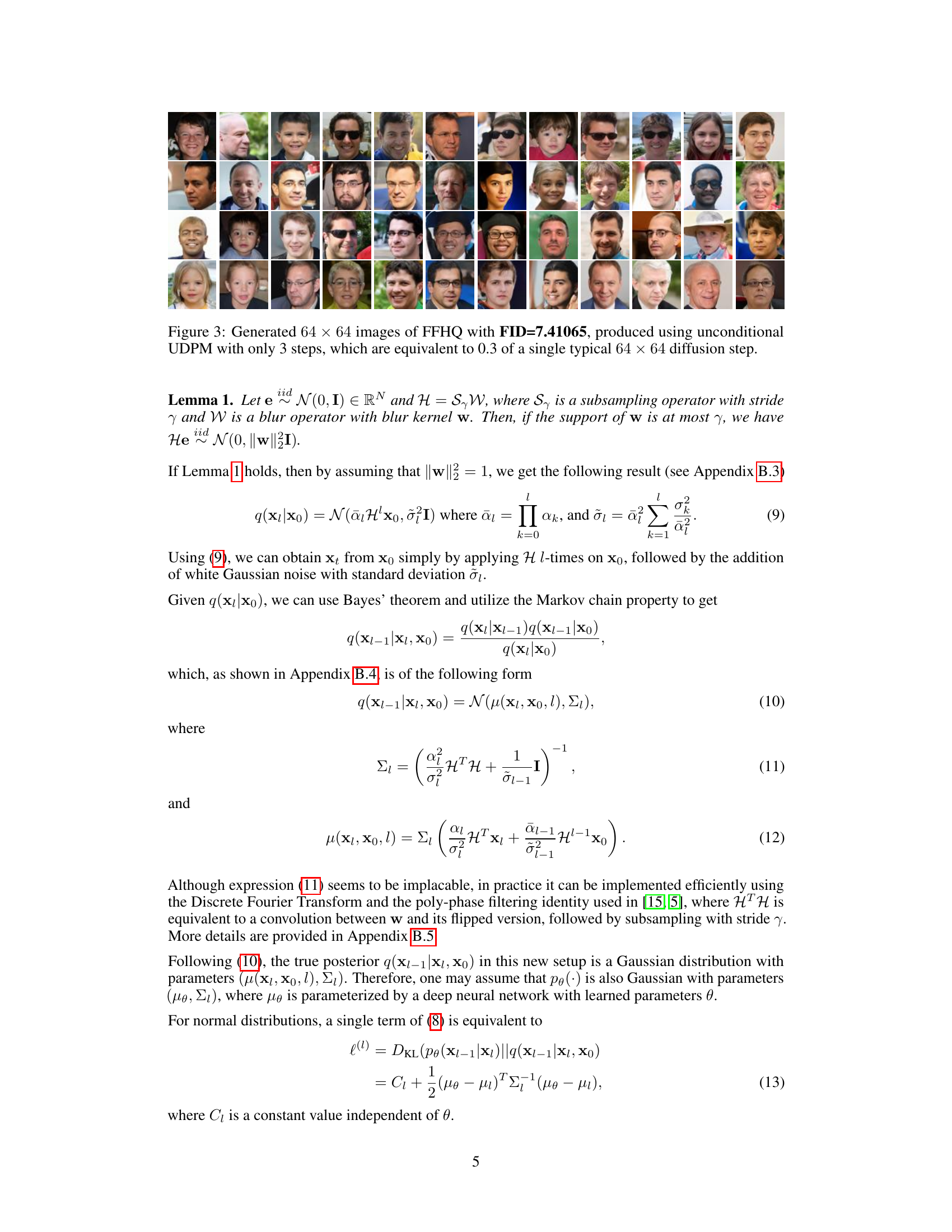
🔼 This figure shows 64 examples of 64x64 images generated from the FFHQ dataset using the proposed UDPM model. The model only required 3 diffusion steps, which is significantly fewer than traditional diffusion models. The FID score of 7.41065 indicates high-quality image generation.
read the caption
Figure 3: Generated 64 × 64 images of FFHQ with FID=7.41065, produced using unconditional UDPM with only 3 steps, which are equivalent to 0.3 of a single typical 64 × 64 diffusion step.
🔼 This figure illustrates the forward and reverse diffusion processes in the proposed Upsampling Diffusion Probabilistic Model (UDPM). The forward process starts with data samples (X0) and iteratively adds noise while simultaneously downsampling the latent variables (X1, X2, X3). Conversely, the reverse process starts with pure noise (XL) and gradually denoises and upsamples the latent variables to reconstruct the data samples (X0). This contrasts with traditional DDPMs that only add noise and do not downsample, resulting in a more efficient generation process.
read the caption
Figure 1: The Upsampling Diffusion Probabilistic Model (UDPM) scheme for 3 diffusion steps (L = 3). In addition to the gradual noise perturbation in traditional DDPMs, UDPM also downsamples the latent variables. Accordingly, in the reverse process, UDPM denoises and upsamples the latent variables to generate images from the data distribution.

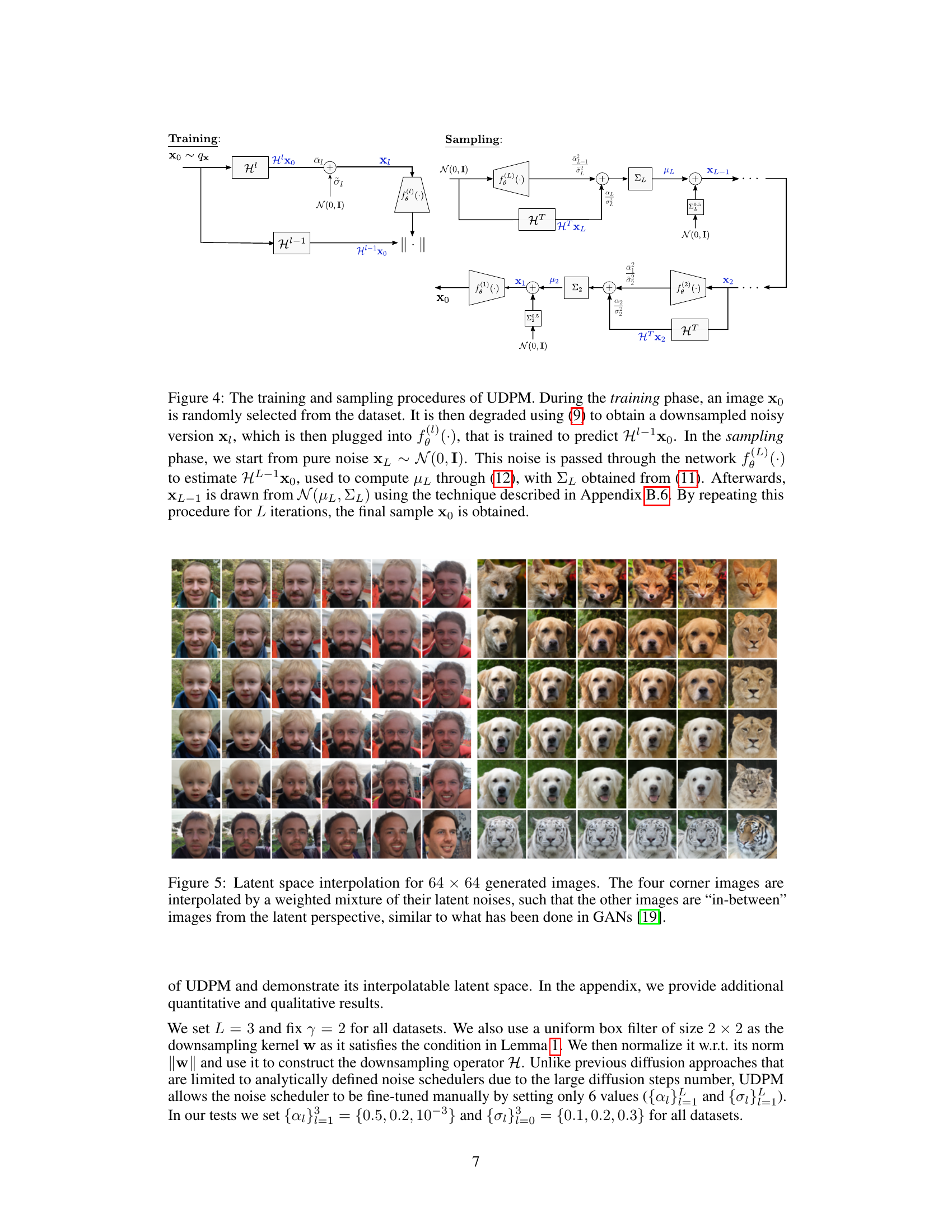
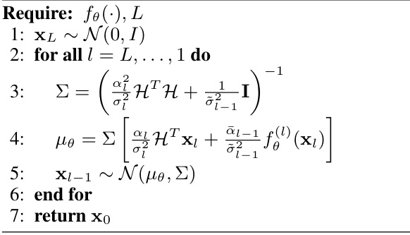
🔼 This figure illustrates the training and sampling processes of the Upsampling Diffusion Probabilistic Model (UDPM). The training process involves downsampling an image using a blur filter and subsampling, adding noise, and training a neural network to predict the original image from the noisy, downsampled version. The sampling process begins with pure noise and iteratively upsamples and denoises the image using the trained network to generate a sample from the data distribution.
read the caption
Figure 4: The training and sampling procedures of UDPM. During the training phase, an image x0 is randomly selected from the dataset. It is then degraded using (9) to obtain a downsampled noisy version x1, which is then plugged into f(L)(.), that is trained to predict HL−1x0. In the sampling phase, we start from pure noise xL ~ N(0, I). This noise is passed through the network f(L)(.) to estimate HL−1x0, used to compute μ1 through (12), with Σ1 obtained from (11). Afterwards, xL−1 is drawn from N(μ1, Σ1) using the technique described in Appendix B.6. By repeating this procedure for L iterations, the final sample x0 is obtained.
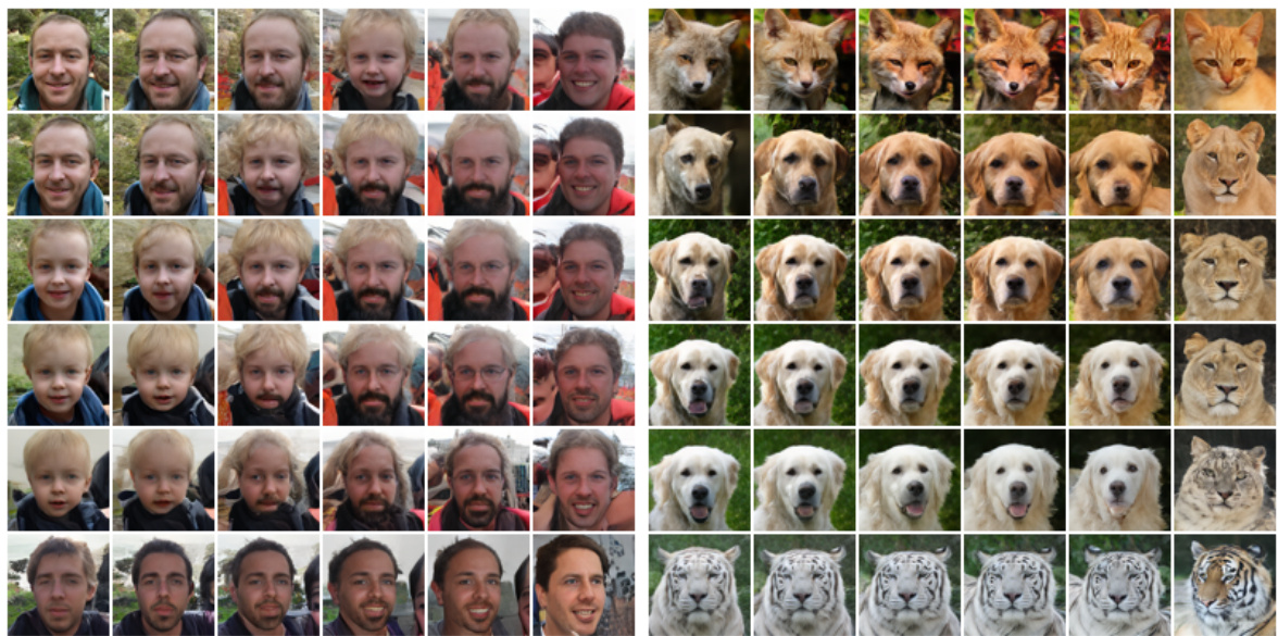
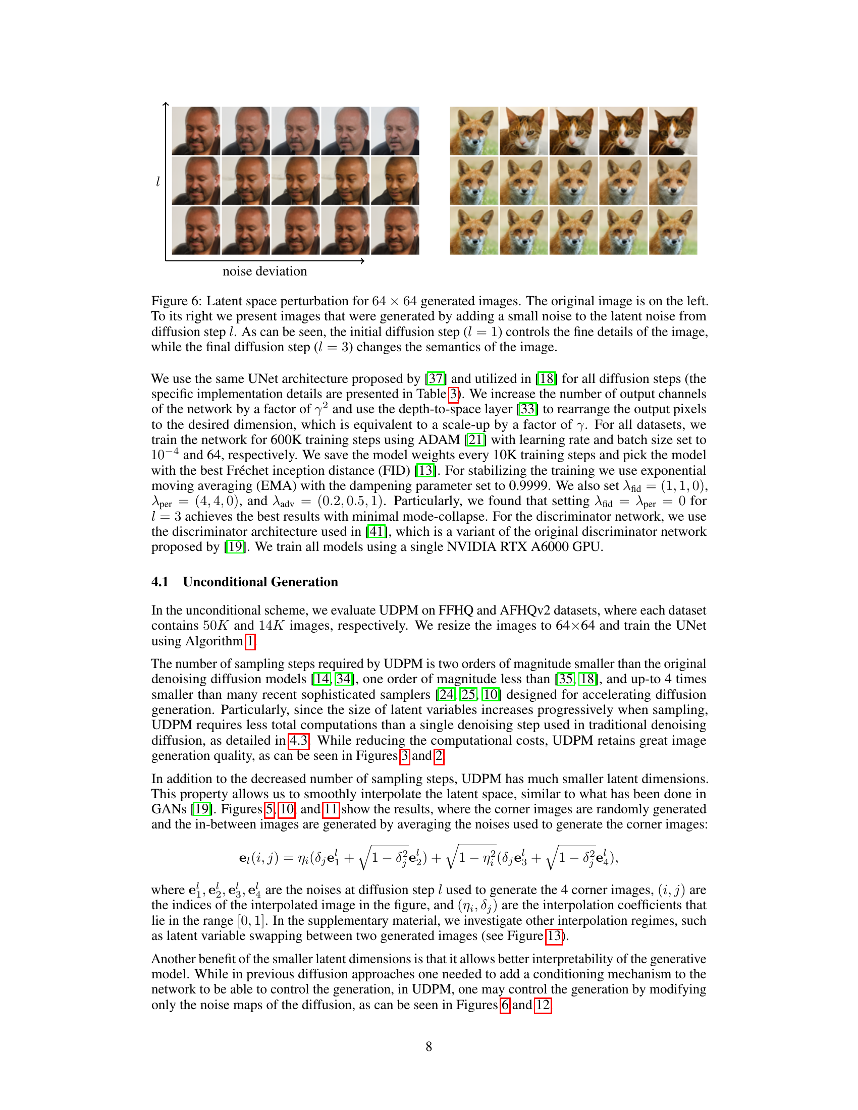
🔼 This figure shows the results of latent space interpolation using UDPM. Four corner images are generated, and the intervening images are created by weighted mixtures of the corner images’ latent noise. This demonstrates the model’s ability to generate images that smoothly transition between different styles.
read the caption
Figure 5: Latent space interpolation for 64 × 64 generated images. The four corner images are interpolated by a weighted mixture of their latent noises, such that the other images are “in-between” images from the latent perspective, similar to what has been done in GANs [19].

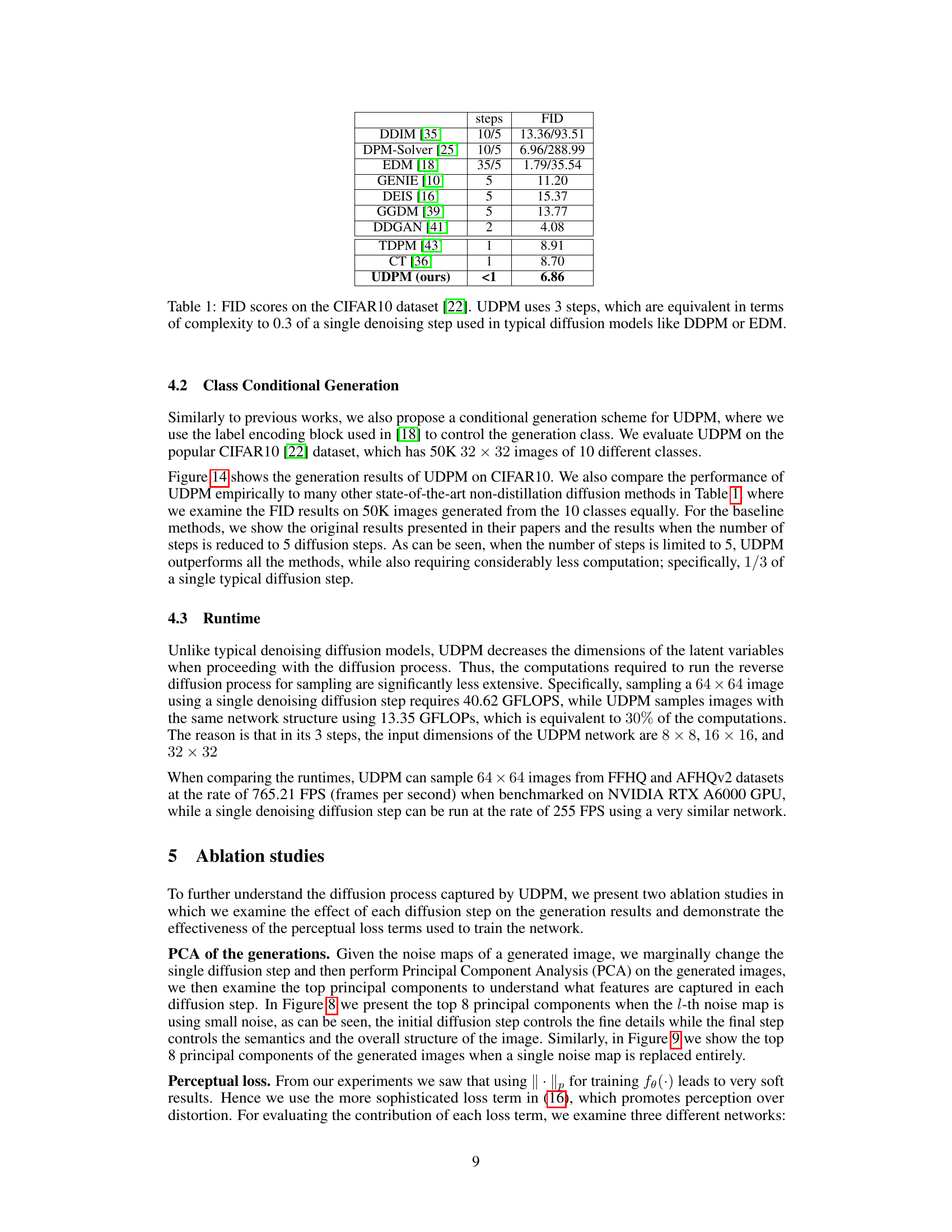
🔼 This figure shows the results of latent space interpolation in the UDPM model. Four corner images (different faces and animals) were generated using UDPM. The images in between these corners are generated by taking a weighted average of the latent noise vectors used to generate the corners. This demonstrates the UDPM model’s ability to smoothly interpolate between different image samples in latent space, similar to what is possible with GANs. This highlights the interpretability of UDPM’s latent space.
read the caption
Figure 5: Latent space interpolation for 64 × 64 generated images. The four corner images are interpolated by a weighted mixture of their latent noises, such that the other images are “in-between” images from the latent perspective, similar to what has been done in GANs [19].

🔼 This figure shows the impact of different loss functions on the quality of generated images using the FFHQ64 dataset. Three different models were trained with different combinations of loss terms: (1) l1 + lper + ladv (using all three loss terms, l1 loss, perceptual loss, and adversarial loss), (2) l1 + lper (using l1 loss and perceptual loss), and (3) l1 (only using l1 loss). The results demonstrate that incorporating both perceptual and adversarial loss functions significantly improves the quality of generated images, as evidenced by the lower FID scores (Fréchet Inception Distance), and visual inspection of the generated images. Lower FID scores indicate better image quality.
read the caption
Figure 7: Visual comparison of the loss terms effect on the FFHQ64 dataset generation results.

🔼 This figure shows the top 8 principal components of a covariance matrix. The matrix was calculated from 128 images. These images were generated using a diffusion model. Two of the diffusion steps were fixed and a small amount of noise was added to the third step. Each row of images represents the principal components of the covariance matrix for a different diffusion step. This visualization helps to understand how the different diffusion steps affect the generated images.
read the caption
Figure 8: The first 8 principal components of the covariance matrix computed over 128 images generated by fixing two diffusion steps and adding small perturbation noise to the third (indexed above).
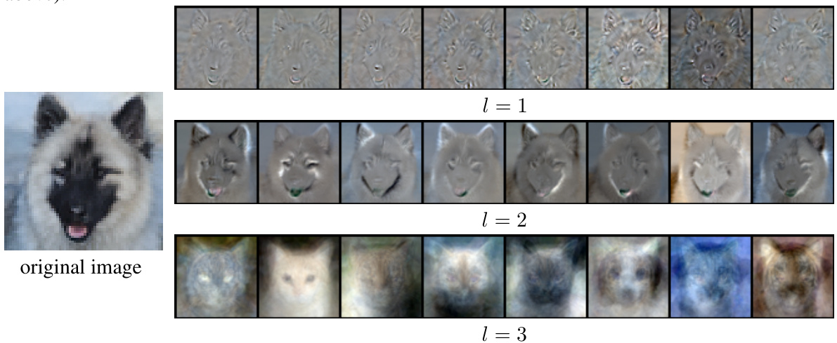
🔼 This figure illustrates the process of the Upsampling Diffusion Probabilistic Model (UDPM). It shows the forward diffusion process, where noise is gradually added to an image while simultaneously downsampling the latent representation. This is followed by the reverse process, where the model denoises and upsamples the latent representation to reconstruct the original image. The figure highlights the key difference between UDPM and traditional DDPMs: the incorporation of downsampling in the forward pass.
read the caption
Figure 1: The Upsampling Diffusion Probabilistic Model (UDPM) scheme for 3 diffusion steps (L = 3). In addition to the gradual noise perturbation in traditional DDPMs, UDPM also downsamples the latent variables. Accordingly, in the reverse process, UDPM denoises and upsamples the latent variables to generate images from the data distribution.

🔼 This figure shows an example of latent space interpolation in the AFHQv2 dataset using the proposed UDPM model. Four corner images are selected, and their latent noise vectors are linearly interpolated to create intermediate images. The resulting images demonstrate the model’s ability to generate smooth transitions between different image features in the latent space, showcasing its ability to create meaningful interpolations.
read the caption
Figure 10: AFHQv2 [6] latent space interpolation example. The four corner images are interpolated by a weighted mixture of their latent noises, such that the other images are “in-between” images from the latent perspective, similar to what has been done in GANs [19]. All the images are of size 64 × 64.

🔼 This figure demonstrates the ability of the UDPM model to perform latent space interpolation. Four corner images were generated, and then intermediate images were created by blending the latent noise vectors of the corner images. The result shows a smooth transition between images, indicating a well-structured and continuous latent space that supports meaningful interpolations.
read the caption
Figure 5: Latent space interpolation for 64 × 64 generated images. The four corner images are interpolated by a weighted mixture of their latent noises, such that the other images are “in-between” images from the latent perspective, similar to what has been done in GANs [19].
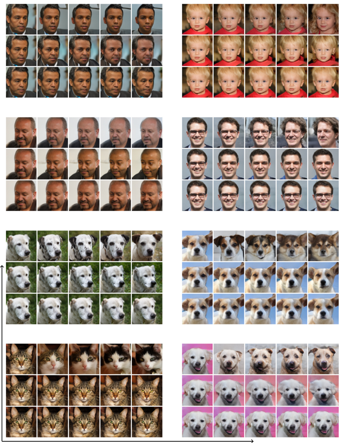
🔼 This figure shows the results of latent space interpolation. Four corner images are generated, and the other images are generated by interpolating the latent noise of the corner images. This demonstrates the model’s ability to smoothly transition between different image styles in the latent space, similar to GANs.
read the caption
Figure 5: Latent space interpolation for 64 × 64 generated images. The four corner images are interpolated by a weighted mixture of their latent noises, such that the other images are “in-between” images from the latent perspective, similar to what has been done in GANs [19].
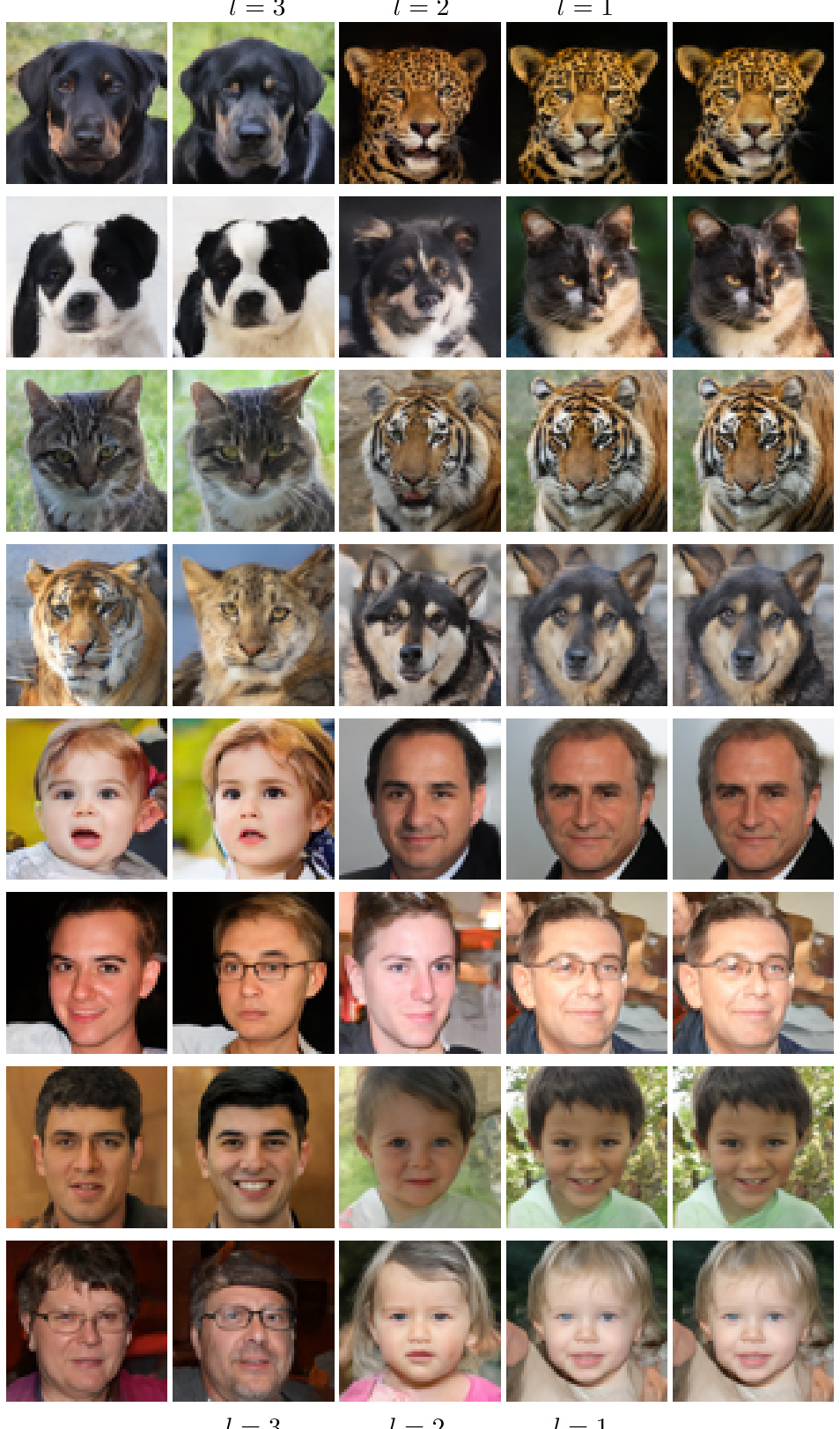
🔼 This figure demonstrates the effect of swapping latent variables (noise maps) between two generated images. By replacing the noise map from one image with the corresponding noise map from another at each diffusion step (l=1,2,3), the figure shows how the change at each step affects the final generated image. This illustrates the impact of different noise levels at various stages of the generation process and highlights the model’s ability to interpret and manipulate intermediate representations.
read the caption
Figure 13: Latent variable swapping: Given the left and right images with the noise maps used for generating them, we replace the l-th noise map of the image on the right with the l-th noise map of the image on the left to see how each diffusion step affect the result (middle columns).

🔼 This figure shows 100 sample images generated from the CIFAR10 dataset using the proposed conditional Upsampling Diffusion Probabilistic Model (UDPM). The model only requires 3 diffusion steps to generate these images, which is significantly less than traditional diffusion models. Each image is 32x32 pixels and represents one of the 10 classes in the CIFAR10 dataset.
read the caption
Figure 14: Generated 32 × 32 images of CIFAR10 [22] using conditional UDPM, requiring only 3 diffusion steps; equivalent to 0.3 traditional denoising step.
More on tables
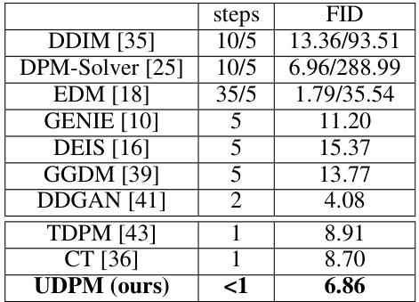
🔼 This table compares the Fréchet Inception Distance (FID) scores of UDPM against other state-of-the-art diffusion models on the CIFAR10 dataset. It highlights UDPM’s superior performance, achieving a lower FID score with significantly fewer steps (3) than other models, which require 1 to 35 steps. The table emphasizes that UDPM’s 3 steps are computationally equivalent to just 0.3 of a single step in traditional diffusion models, showcasing its efficiency.
read the caption
Table 1: FID scores on the CIFAR10 dataset [22]. UDPM uses 3 steps, which are equivalent in terms of complexity to 0.3 of a single denoising step used in typical diffusion models like DDPM or EDM.

🔼 This table compares the Fréchet Inception Distance (FID) scores achieved by UDPM and EDM on the FFHQ and AFHQv2 datasets. FID is a metric used to evaluate the quality of generated images, with lower scores indicating better quality. The table highlights that UDPM achieves comparable or better FID scores with significantly fewer computational steps. Specifically, UDPM’s 3 steps are equivalent to only 0.3 steps of the EDM model, showcasing UDPM’s computational efficiency.
read the caption
Table 2: FID scores comparison between UDPM and EDM [18] on the FFHQ [19] and AFHQv2 [6] datasets. UDPM requires 3 diffusion steps, which is equivalent to 0.3 denoising steps of EDM.

🔼 This table presents the hyperparameters used during the training phase of the UDPM model for three different datasets: CIFAR10, AFHQv2, and FFHQ. The hyperparameters include the learning rate, the number of warmup steps, batch size, dropout rate, optimizer used (Adam), and the number of GPUs used for training. These settings were optimized for each dataset to achieve the best results.
read the caption
Table 3: Training hyperparameters.
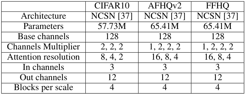
🔼 This table shows the hyperparameters used for the different datasets in the UDPM model. These hyperparameters control various aspects of the model’s architecture and training, such as the number of channels, the attention resolution, and the number of blocks per scale. Different datasets may require different hyperparameter settings to achieve optimal performance.
read the caption
Table 4: Model hyperparameters.

🔼 This table details the hyperparameters used for the discriminator network in the UDPM model, categorized by dataset (CIFAR10, AFHQv2, FFHQ). The hyperparameters include the discriminator architecture (DDGAN [41]), the number of parameters, the number of channels at each layer, the number of input channels, the number of blocks per scale, the type of blocks used (NCSN down), the gradient penalty weight (from [41]), and the dropout rate.
read the caption
Table 5: Discriminator network hyperparameters.
Full paper#
