TL;DR#
The training dynamics of neural networks are often categorized into “lazy” and “active” regimes, each with its strengths and weaknesses. The lazy regime features simpler, linear dynamics, but lacks the feature learning capability of active regimes. Conversely, the active regime is characterized by complex, nonlinear dynamics and feature learning, but struggles with slow convergence and can get stuck in poor solutions. This dichotomy has limited our understanding of the training process and optimization strategies.
This paper introduces a unifying framework that captures both regimes and also reveals an intermediate “mixed” regime. The core contribution is a novel formula that elegantly describes the evolution of the network’s learned matrix. This formula explains how the network can simultaneously leverage the simplicity of lazy dynamics for smaller singular values and the feature learning power of active dynamics for larger values, thus combining the advantages of both and addressing the limitations of each regime. This leads to a more complete understanding of neural network training and opens up new avenues for designing better optimization algorithms.
Key Takeaways#
Why does it matter?#
This paper is crucial because it bridges the gap between two dominant paradigms in neural network training: the lazy and active regimes. By providing a unified framework, it enhances our understanding of training dynamics and opens new avenues for optimization strategies, particularly in scenarios requiring both rapid convergence and low-rank solutions.
Visual Insights#

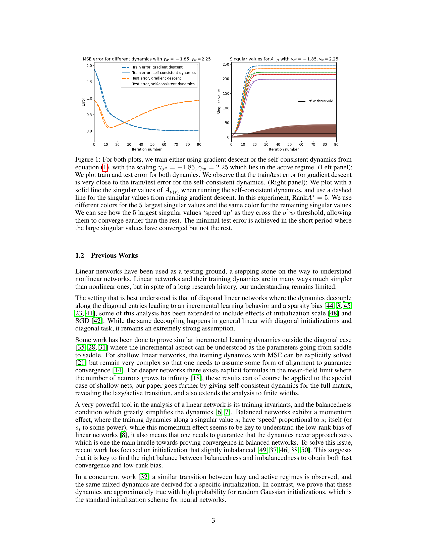
🔼 This figure compares the training and testing error curves obtained using gradient descent and the self-consistent dynamics proposed in the paper, when the scaling parameters are set to γσ2 = -1.85 and γω = 2.25, which corresponds to the active regime. The left panel shows that both methods yield similar training and testing error curves. The right panel shows the evolution of singular values for Ae(t), where the five largest singular values converge faster once they cross the σ²w threshold.
read the caption
Figure 1: For both plots, we train either using gradient descent or the self-consistent dynamics from equation (1), with the scaling γσ2 = -1.85, γω = 2.25 which lies in the active regime. (Left panel): We plot train and test error for both dynamics. We observe that the train/test error for gradient descent is very close to the train/test error for the self-consistent dynamics. (Right panel): We plot with a solid line the singular values of Ae(t) when running the self-consistent dynamics, and use a dashed line for the singular values from running gradient descent. In this experiment, RankA* = 5. We use different colors for the 5 largest singular values and the same color for the remaining singular values. We can see how the 5 largest singular values ‘speed up’ as they cross the σ²w threshold, allowing them to converge earlier than the rest. The minimal test error is achieved in the short period where the large singular values have converged but not the rest.
Full paper#

