TL;DR#
Generating realistic graphs that adhere to real-world constraints is crucial for many applications, but existing methods struggle to guarantee these constraints. Current graph generation techniques often produce invalid graphs, hindering their use in practical applications. This is especially problematic when domain-specific knowledge, like planarity in digital pathology, is essential.
ConStruct is a novel framework that integrates hard structural constraints into graph diffusion models. It employs an edge-absorbing noise model and a projector operator to ensure the generated graphs consistently satisfy the specified properties. The method shows impressive versatility across multiple constraints and achieves state-of-the-art performance on various benchmarks. Its application to real-world datasets, such as digital pathology graphs, demonstrates significant improvement in data validity.
Key Takeaways#
Why does it matter?#
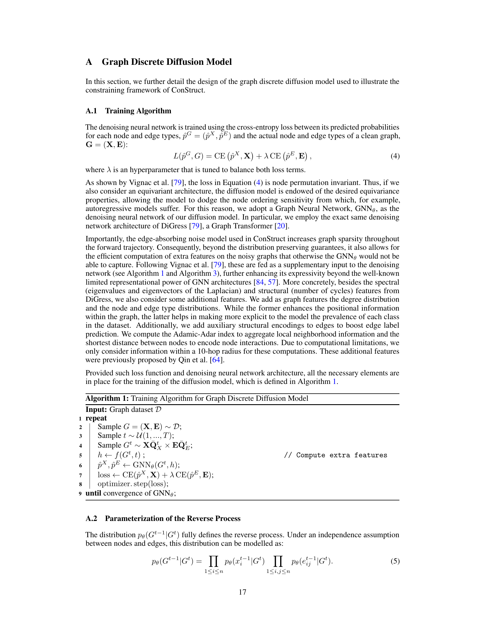
This paper is crucial for researchers in graph generation and related fields because it introduces a novel framework, ConStruct, that effectively addresses the challenge of incorporating domain knowledge into graph generation models. This significantly enhances the quality and validity of generated graphs, leading to improved results in various applications. The method’s versatility and high performance across various structural constraints make it highly valuable for researchers working on diverse real-world problems involving graphs.
Visual Insights#

🔼 This figure illustrates the Constrained Graph Discrete Diffusion framework proposed in the paper. The framework consists of a forward diffusion process (where noise is progressively added to the graph) and a reverse diffusion process (where the noise is removed to generate a new graph). The key innovation is the inclusion of a ‘projector’ that ensures generated graphs always adhere to specified structural constraints (in this case, acyclicity). The forward process uses an edge-absorbing noise model, and the reverse process uses a GNN to predict and insert edges while the projector removes any edge insertions which would violate the constraints.
read the caption
Figure 1: Constrained graph discrete diffusion framework. The forward process consists of an edge deletion process driven by the edge-absorbing noise model, while the node types may switch according to the marginal noise model. At sampling time, the projector operator ensures that sampled graphs remain within the constrained domain throughout the entire reverse process. In the illustrated example, the constrained domain consists exclusively of graphs with no cycles. We highlight in gray the components responsible for preserving the constraining property.
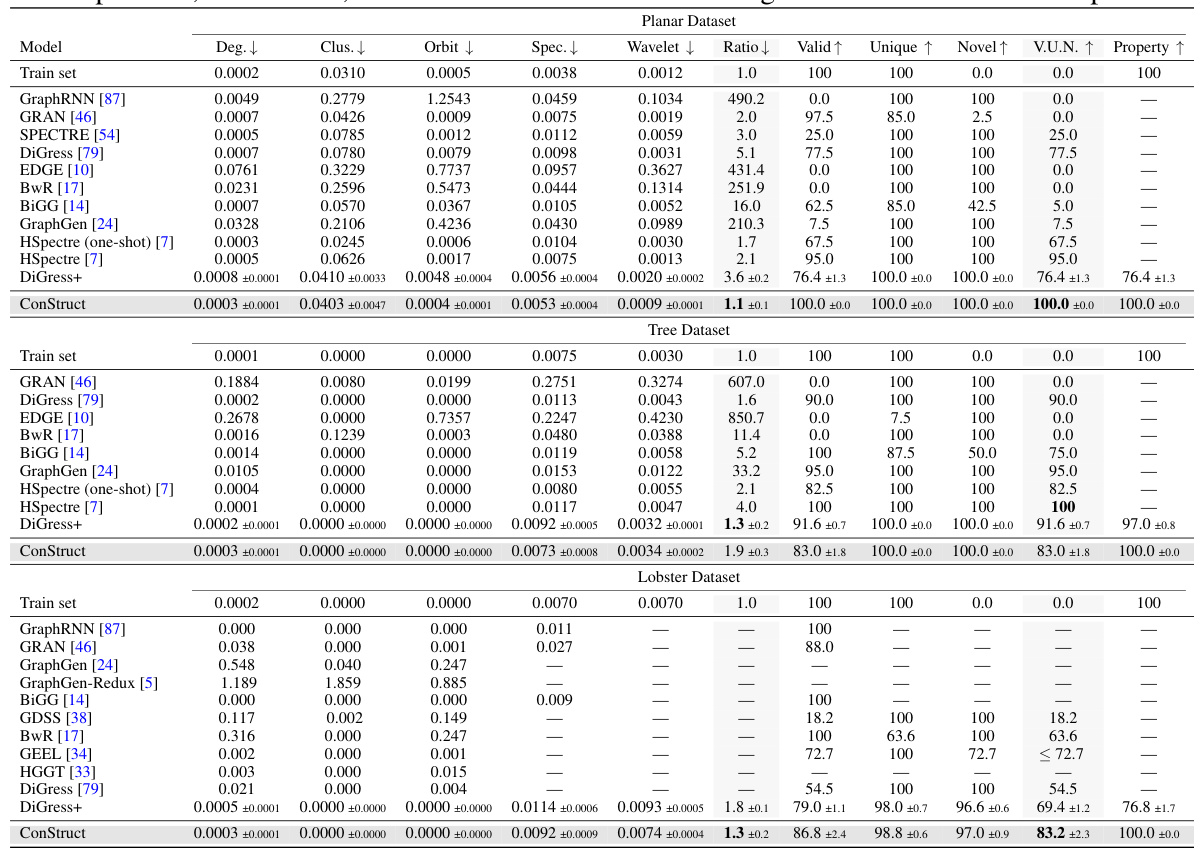
🔼 This table presents a quantitative comparison of different graph generation models on three synthetic datasets: planar, tree, and lobster graphs. The models are evaluated using several metrics, including those measuring the similarity of generated graphs to the training data distribution, the uniqueness and novelty of the generated samples, their validity in terms of satisfying structural constraints, and the overall success of the models in satisfying the target structural properties. The results are presented as mean ± standard error across five sampling runs of 100 graphs each. The table also references the source papers for the results of the baseline models, allowing for reproducibility.
read the caption
Table 1: Graph generation performance on synthetic graphs. We present the results over five sampling runs of 100 generated graphs each, in the format mean ± standard error of the mean. The remaining values are retrieved from Bergmeister et al. [7] for the planar and tree datasets, and from Dai et al. [14] and Jang et al. [34] for the lobster dataset. For the average ratio computation, we follow [7] and do not consider the metrics whose train set MMD is 0. We recompute the train set MMDs according to our splits but, for fairness, in the retrieved methods the average ratio metric is not recomputed.
In-depth insights#
Constrained Graph Diffusion#
Constrained graph diffusion presents a novel approach to address the limitations of traditional graph diffusion models in generating graphs that adhere to specific structural properties. The core idea revolves around integrating hard constraints into the diffusion process, ensuring that sampled graphs remain within a predefined domain throughout the entire trajectory, in both forward and reverse diffusion steps. This is achieved by introducing an edge-absorbing noise model and a projector operator. The edge-absorbing noise model facilitates the forward diffusion process as an edge deletion process, which is crucial for preserving structural properties during noise injection. The projector operator, in turn, guarantees that the reverse diffusion process generates graphs that satisfy the specified property by refining the sampled graphs and discarding any edge insertions that violate the constraints. The versatility of the method is demonstrated through various constraints, including planarity and acyclicity, and its superior performance is showcased on both synthetic and real-world datasets. The significance of Constrained graph diffusion lies in its ability to incorporate domain expertise into generative models, leading to more meaningful and realistic graph generation, especially relevant in applications like digital pathology and molecular design where invalid graphs can hinder deployment.
ConStruct Framework#
The ConStruct framework presents a novel approach to integrating hard constraints into graph diffusion models for graph generation. This is crucial because real-world applications often require generated graphs to adhere to specific structural properties (e.g., planarity in digital pathology). ConStruct’s core innovation is the use of an edge-absorbing noise model and a projector operator. The noise model ensures that the forward diffusion process, which involves progressively adding noise, maintains the desired structural properties. The projector then acts during the reverse process, ensuring that edges added during denoising do not violate constraints. This guarantees that sampled graphs remain within the valid domain throughout the entire generative process, a significant improvement over existing conditioned or unconstrained methods. The framework’s versatility is demonstrated through its application to diverse constraints such as planarity, acyclicity, and lobster components, achieving state-of-the-art performance in various benchmark datasets and a real-world digital pathology application. ConStruct’s theoretical foundation lies in its edge-deletion invariant constraint design, making it highly effective for a broad class of structural properties. The implementation also incorporates efficiency improvements such as incremental algorithms and a blocking edge hash table. This combination of theoretical rigor, practical applicability, and efficiency enhancements makes the ConStruct framework a significant advancement in the field of constrained graph generation.
Edge-Del Aware Forward#
The heading ‘Edge-Del Aware Forward’ suggests a process within a graph generative model. The core idea is to incorporate domain knowledge, specifically about structural properties preserved under edge deletion, into the forward diffusion process. The forward process is designed to be an edge deletion process, ensuring that the resulting noisy graph retains the desired structural properties at every step. This contrasts with traditional methods where the forward process might generate graphs violating these properties, requiring costly post-processing or rejection. By making the forward process edge-deletion aware, the model learns to inherently respect the structural constraints, simplifying the process and leading to improved performance and validity of the generated graphs. This approach offers a key advantage in applications where the structural properties are critical for the generated graph’s practical utility. The ‘Edge-Del Aware Forward’ process is a crucial component of a broader framework that also likely utilizes a reverse process to refine the noisy graphs back to realistic, constrained structures. This methodology is innovative because it directly addresses the challenge of incorporating domain knowledge into graph generative models by intelligently designing the noise model within the diffusion process.
Projector Operator#
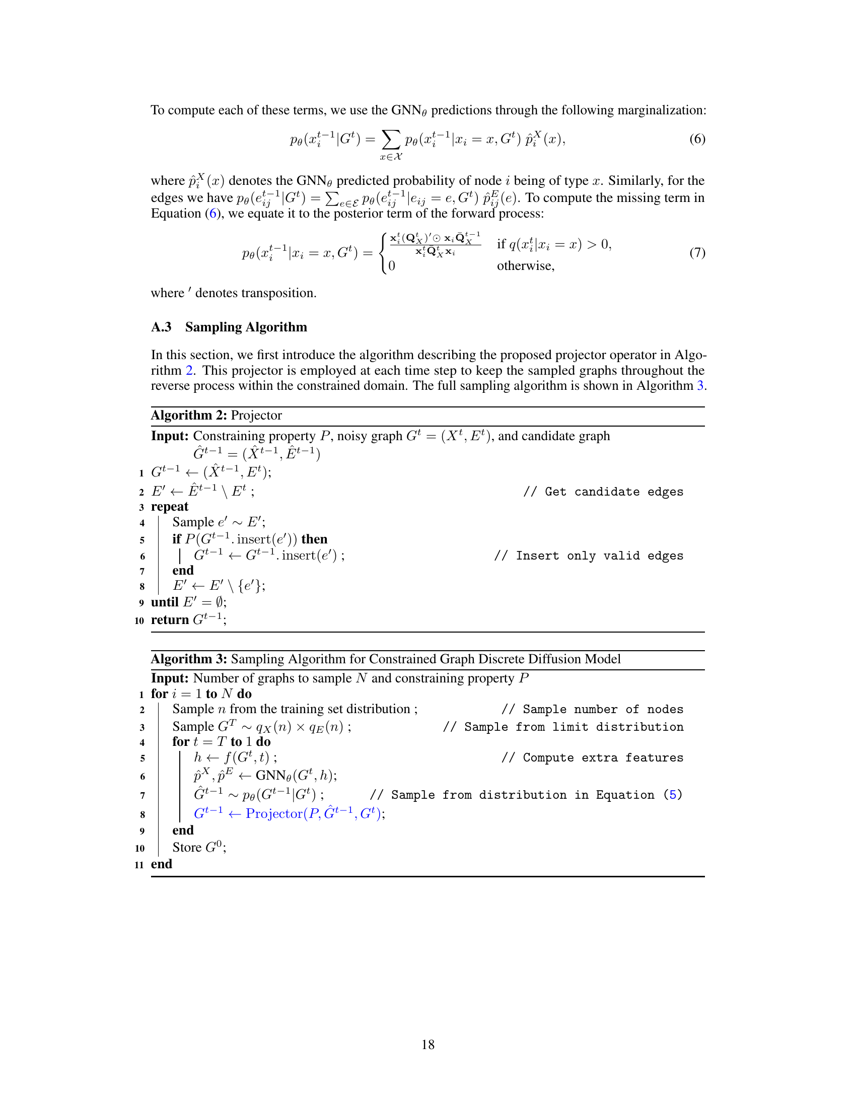
The Projector Operator is a crucial component in the ConStruct framework, addressing the challenge of incorporating hard constraints into graph diffusion models. Its function is to guarantee that sampled graphs remain within the desired domain throughout the reverse diffusion process, ensuring the generation of valid graphs that adhere to specified structural properties like planarity or acyclicity. The operator achieves this by acting as a filter, selectively inserting edges suggested by the diffusion model while rejecting any that would violate the constraints. This selective edge insertion is achieved through an iterative process, examining each candidate edge and confirming its compatibility with the structural constraints before accepting it. By strategically incorporating this projector, ConStruct overcomes the limitations of standard conditioned graph generation approaches and enables the creation of high-quality, structurally-valid graphs across various domains.
Future Directions#
The paper’s “Future Directions” section would ideally expand on the limitations of ConStruct, specifically its restriction to edge-deletion invariant properties. Exploring extensions to encompass edge-insertion invariant properties would broaden the applicability to a wider range of real-world scenarios and structural constraints. Addressing the scalability challenges presented by the edge-absorbing noise model, and the computational cost of the projector for large graphs is crucial for practical applications. Further exploration of alternative noise models and the development of more efficient projection algorithms are necessary to improve performance. Finally, investigating the combination of ConStruct with other generative models or incorporating different types of constraints is a promising area of research, as is exploring the use of ConStruct for problems beyond graph generation. The potential for integrating this framework into other modalities such as sequential data or high-dimensional data should also be considered.
More visual insights#
More on figures

🔼 This figure illustrates the projector operator used in ConStruct’s reverse process. It shows how, given a noisy graph Gt and a candidate denoised graph Gt-1 sampled from the diffusion model, the projector iteratively inserts candidate edges, discarding any that would violate the target property (e.g., acyclicity, as shown in the example). This ensures that the final sampled graph Gt-1 is guaranteed to satisfy the property. The gray components highlight which parts are responsible for preserving the desired property.
read the caption
Figure 2: Projector operator. At each iteration, we start by sampling a candidate graph Gt-1 from the distribution pe(Gt-1|Gt) provided by the diffusion model. Then, the projector step inserts in an uniformly random manner the candidate edges, discarding those that violate the target property, P, i.e., acyclicity in this illustration. In the end of the reverse step, we find a graph Gt-1 that is guaranteed to comply with such property.

🔼 This figure shows the process of extracting a subgraph representing tertiary lymphoid structures (TLSs) from a larger whole-slide image (WSI) graph. The left panel displays the full WSI graph, where nodes represent cells and edges represent cell-cell interactions. A specific region containing a TLS is highlighted in a circle. The middle panel shows the extracted subgraph, focusing on the cells and interactions within the TLS. The right panel illustrates the TLS embedding, which quantifies the TLS content based on edge types (interactions between different cell types). The different colors represent different cell types, with the presence of a cluster of B-cells surrounded by supporting T-cells indicating a high TLS content.
read the caption
Figure 4: Extraction of a cell subgraph (center) from a WSI graph (left). From this cell subgraph, we can then compute the TLS embedding based on the classification of the edges into different categories, shown on the right. We can observe a cluster of B-cells surrounded by some support T-cells, characteristic of a high TLS content.

🔼 This figure illustrates the ConStruct framework for constrained graph generation using discrete diffusion models. The forward process involves progressively adding noise to a graph by deleting edges and potentially changing node types. The reverse process then recovers a clean graph, but with the crucial addition of a ‘projector’ which ensures the generated graphs adhere to pre-defined structural constraints (e.g., no cycles, planarity). The projector acts by rejecting any edge additions that would violate these constraints during the reverse diffusion process.
read the caption
Figure 1: Constrained graph discrete diffusion framework. The forward process consists of an edge deletion process driven by the edge-absorbing noise model, while the node types may switch according to the marginal noise model. At sampling time, the projector operator ensures that sampled graphs remain within the constrained domain throughout the entire reverse process. In the illustrated example, the constrained domain consists exclusively of graphs with no cycles. We highlight in gray the components responsible for preserving the constraining property.

🔼 This figure illustrates the ConStruct framework for constrained graph generation using discrete diffusion models. The forward process involves progressively adding noise to a graph by deleting edges and potentially changing node types. The reverse process then aims to reconstruct a clean graph, but with the constraint that the generated graph always satisfies a given property (e.g., acyclicity in the example). The projector operator ensures the generated graph stays within the allowed domain throughout this reverse process.
read the caption
Figure 1: Constrained graph discrete diffusion framework. The forward process consists of an edge deletion process driven by the edge-absorbing noise model, while the node types may switch according to the marginal noise model. At sampling time, the projector operator ensures that sampled graphs remain within the constrained domain throughout the entire reverse process. In the illustrated example, the constrained domain consists exclusively of graphs with no cycles. We highlight in gray the components responsible for preserving the constraining property.
🔼 This figure visualizes intermediate steps in the reverse process of the ConStruct model for three different types of graphs: planar, tree, and lobster. Each row represents a graph type. Each column shows the graph at different stages of the reverse process, starting from a noisy graph (t=T) on the left and ending with a clean graph (t=1) on the right. Green edges represent edges added by the diffusion model that satisfy the constraints, while red edges are discarded by the projector because they would violate the constraints.
read the caption
Figure 12: Visualizations of intermediate graphs throughout the reverse process. The notation follows the one of the rest of the paper: we obtain Gt-1 after applying the projector on Ĝt−1, which in turn is obtained from Gt through the diffusion model. From the new edges obtained in Gt-1, we color them in green when they do not break the constraining property and in red otherwise. We can observe that the red edges are rejected. To better emphasize the edge rejection by the projector, we do not use a fully trained model and use a trajectory length, T, smaller than usual, resulting in less accurate edge predictions.
🔼 This figure shows the reverse process of ConStruct for generating low and high TLS content graphs. The process begins with a graph having no edges (t=T) and gradually adds edges in the reverse diffusion process (moving from t=T to t=0). The color of nodes indicates different cell phenotypes, demonstrating how the noise model affects node types and the projector ensures that generated graphs maintain the correct structure.
read the caption
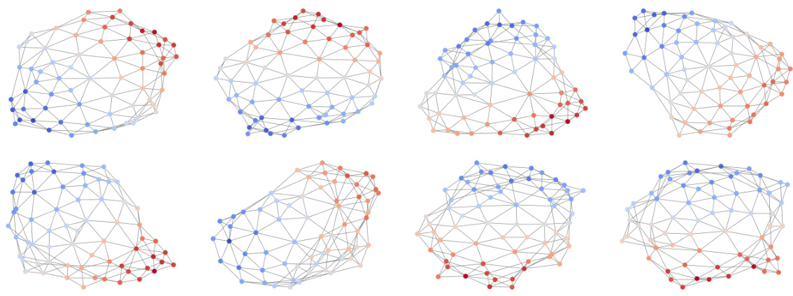
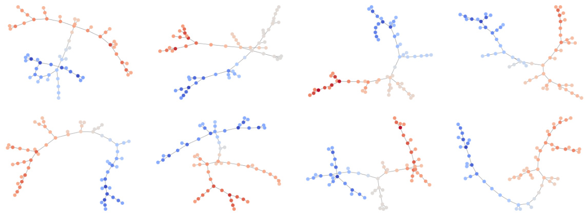
Figure 11: Reverse processes for generation of low (top) and high (bottom) TLS content graphs using ConStruct. We start from a graph without any edge on the left (t = T) and progressively build the graph, as a consequence of the absorbing noise model. The node types switch along the trajectory due to the marginal noise model. On the right, we have a fresh new sample (t = 0). The phenotypes color key is presented in Figure 4.
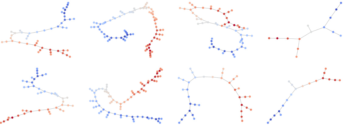
🔼 This figure visualizes the reverse process of ConStruct for generating low and high TLS content graphs. It starts with a graph having no edges (t=T) and iteratively adds edges during the reverse diffusion process. The node types also change throughout this process. The right side shows the final generated graph (t=0).
read the caption
Figure 11: Reverse processes for generation of low (top) and high (bottom) TLS content graphs using ConStruct. We start from a graph without any edge on the left (t = T) and progressively build the graph, as a consequence of the absorbing noise model. The node types switch along the trajectory due to the marginal noise model. On the right, we have a fresh new sample (t = 0). The phenotypes color key is presented in Figure 4.

🔼 This figure illustrates the ConStruct framework for constrained graph generation using discrete diffusion models. The forward process involves progressively adding noise to a graph by deleting edges and potentially changing node types. The reverse process uses a neural network and a projector operator to reconstruct a clean graph from the noisy version, while simultaneously ensuring that the generated graphs satisfy the specified constraints. The example shown highlights the generation of cycle-free graphs.
read the caption
Figure 1: Constrained graph discrete diffusion framework. The forward process consists of an edge deletion process driven by the edge-absorbing noise model, while the node types may switch according to the marginal noise model. At sampling time, the projector operator ensures that sampled graphs remain within the constrained domain throughout the entire reverse process. In the illustrated example, the constrained domain consists exclusively of graphs with no cycles. We highlight in gray the components responsible for preserving the constraining property.
🔼 This figure illustrates the ConStruct framework for constrained graph generation using discrete diffusion models. The forward diffusion process involves an edge-absorbing noise model that progressively deletes edges from the graph. Node types may also change during this forward process. The reverse process reconstructs the graph from noise. A key component is the projector, which ensures that all sampled graphs during the reverse process adhere to the specified structural constraints (in this example, the absence of cycles). The grayed components highlight the parts of the model that specifically maintain the constraints.
read the caption
Figure 1: Constrained graph discrete diffusion framework. The forward process consists of an edge deletion process driven by the edge-absorbing noise model, while the node types may switch according to the marginal noise model. At sampling time, the projector operator ensures that sampled graphs remain within the constrained domain throughout the entire reverse process. In the illustrated example, the constrained domain consists exclusively of graphs with no cycles. We highlight in gray the components responsible for preserving the constraining property.

🔼 This figure visualizes the intermediate steps during the reverse process of the ConStruct model for three different types of graphs (planar, tree, and lobster). It demonstrates how the projector component of the model works by accepting or rejecting candidate edges based on whether they violate the specified structural constraints (planarity, acyclicity, or lobster components). Green edges are accepted, while red edges are rejected because they would violate the constraints. The use of a less-than-fully trained model and a shorter trajectory length (T) was intentional to make the effect of the edge rejection more visually apparent.
read the caption
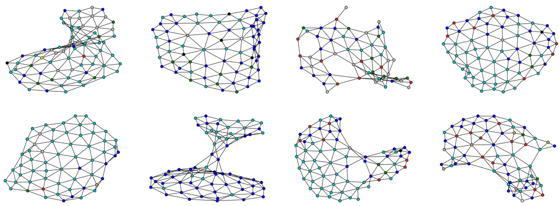
Figure 12: Visualizations of intermediate graphs throughout the reverse process. The notation follows the one of the rest of the paper: we obtain Gt-1 after applying the projector on Ĝt-1, which in turn is obtained from Gt through the diffusion model. From the new edges obtained in Gt-1, we color them in green when they do not break the constraining property and in red otherwise. We can observe that the red edges are rejected. To better emphasize the edge rejection by the projector, we do not use a fully trained model and use a trajectory length, T, smaller than usual, resulting in less accurate edge predictions.

🔼 This figure illustrates the ConStruct framework, which is a novel method for generating graphs with specific structural properties. It depicts the forward and reverse diffusion processes. The forward process involves progressively adding noise to a graph by deleting edges and changing node types. The reverse process then aims to recover the original graph by removing noise, but with a crucial constraint: the projector operator ensures that at each step, the generated graphs satisfy the desired structural property (in this case, acyclicity—no cycles). The gray areas highlight the components designed to maintain these constraints throughout the entire process.
read the caption
Figure 1: Constrained graph discrete diffusion framework. The forward process consists of an edge deletion process driven by the edge-absorbing noise model, while the node types may switch according to the marginal noise model. At sampling time, the projector operator ensures that sampled graphs remain within the constrained domain throughout the entire reverse process. In the illustrated example, the constrained domain consists exclusively of graphs with no cycles. We highlight in gray the components responsible for preserving the constraining property.
More on tables

🔼 This table presents the quantitative results of the proposed ConStruct framework on three different synthetic graph datasets: planar, tree, and lobster. The results are averaged over five runs of 100 generated graphs each and presented as mean ± standard error of the mean. It compares the performance of ConStruct against several existing state-of-the-art graph generation methods across various metrics, including the accuracy of generated graphs in terms of their structural properties (planarity, acyclicity, lobster components) and the similarity of their distributions to the training set (using MMD). The table also shows the percentage of generated graphs that are valid, unique (non-isomorphic), and novel (non-isomorphic to the training set).
read the caption
Table 1: Graph generation performance on synthetic graphs. We present the results over five sampling runs of 100 generated graphs each, in the format mean ± standard error of the mean. The remaining values are retrieved from Bergmeister et al. [7] for the planar and tree datasets, and from Dai et al. [14] and Jang et al. [34] for the lobster dataset. For the average ratio computation, we follow [7] and do not consider the metrics whose train set MMD is 0. We recompute the train set MMDs according to our splits but, for fairness, in the retrieved methods the average ratio metric is not recomputed.

🔼 This table presents the quantitative results of graph generation performance comparison for three different graph datasets: planar, tree, and lobster. For each dataset, multiple metrics are evaluated: Degree, Clustering coefficient, Orbit count, Spectral features, Wavelet transform, and the Average Ratio across the metrics. It also presents the percentage of valid, unique, and novel graphs generated by each method, as well as the overall percentage of graphs satisfying the specific structural constraint of the dataset. The results are presented in the format of mean ± standard error across five sampling runs of 100 generated graphs each. The data for some methods is from previous work and is included for comparison.
read the caption
Table 1: Graph generation performance on synthetic graphs. We present the results over five sampling runs of 100 generated graphs each, in the format mean ± standard error of the mean. The remaining values are retrieved from Bergmeister et al. [7] for the planar and tree datasets, and from Dai et al. [14] and Jang et al. [34] for the lobster dataset. For the average ratio computation, we follow [7] and do not consider the metrics whose train set MMD is 0. We recompute the train set MMDs according to our splits but, for fairness, in the retrieved methods the average ratio metric is not recomputed.

🔼 This table presents a quantitative comparison of ConStruct against other state-of-the-art graph generation models on three synthetic graph datasets: planar, tree, and lobster. For each dataset and model, the table shows the mean and standard error of several graph statistics (degree, clustering coefficient, orbit count, spectral properties, wavelet transform) from 5 runs of 100 generated graphs each. It also shows the proportion of valid, unique, and novel graphs generated, as well as the percentage of graphs that satisfy the target structural property (planarity for planar, acyclicity for tree, and lobster components for lobster). The results are used to evaluate the quality and diversity of generated graphs, demonstrating ConStruct’s ability to generate high-quality graphs that satisfy structural properties.
read the caption
Table 1: Graph generation performance on synthetic graphs. We present the results over five sampling runs of 100 generated graphs each, in the format mean ± standard error of the mean. The remaining values are retrieved from Bergmeister et al. [7] for the planar and tree datasets, and from Dai et al. [14] and Jang et al. [34] for the lobster dataset. For the average ratio computation, we follow [7] and do not consider the metrics whose train set MMD is 0. We recompute the train set MMDs according to our splits but, for fairness, in the retrieved methods the average ratio metric is not recomputed.

🔼 This table presents a quantitative comparison of ConStruct against other state-of-the-art graph generation methods on three synthetic datasets: planar, tree, and lobster. The evaluation metrics include several graph statistics (node degree, clustering coefficient, orbit count, spectral features, wavelet transform features), the average ratio of generated to training set statistics, the proportion of valid, unique, and novel generated graphs, and the proportion of generated graphs satisfying the target property. The results are averaged over five runs of 100 generated graphs per run, and error bars represent the standard error of the mean.
read the caption
Table 1: Graph generation performance on synthetic graphs. We present the results over five sampling runs of 100 generated graphs each, in the format mean ± standard error of the mean. The remaining values are retrieved from Bergmeister et al. [7] for the planar and tree datasets, and from Dai et al. [14] and Jang et al. [34] for the lobster dataset. For the average ratio computation, we follow [7] and do not consider the metrics whose train set MMD is 0. We recompute the train set MMDs according to our splits but, for fairness, in the retrieved methods the average ratio metric is not recomputed.

🔼 This table compares the performance of ConStruct with other state-of-the-art graph generation methods on three synthetic graph datasets: planar, tree, and lobster. For each dataset and method, it shows the mean and standard error of several key metrics (degree, clustering coefficient, orbit count, spectral features, wavelet transform features, and average ratio across metrics). It also includes the percentage of generated graphs that are valid, unique, novel, and satisfy the specific structural constraint. This allows for an assessment of how well each model captures the properties of the target graph distribution while respecting structural properties.
read the caption
Table 1: Graph generation performance on synthetic graphs. We present the results over five sampling runs of 100 generated graphs each, in the format mean ± standard error of the mean. The remaining values are retrieved from Bergmeister et al. [7] for the planar and tree datasets, and from Dai et al. [14] and Jang et al. [34] for the lobster dataset. For the average ratio computation, we follow [7] and do not consider the metrics whose train set MMD is 0. We recompute the train set MMDs according to our splits but, for fairness, in the retrieved methods the average ratio metric is not recomputed.

🔼 This table presents a comparison of different graph generation models on three synthetic datasets: planar, tree, and lobster. The results show various metrics for evaluating graph generation quality, including the Maximum Mean Discrepancy (MMD) for several graph statistics (degree, clustering coefficient, orbit count, spectral properties, wavelet transform) and the proportion of valid, unique, and novel graphs generated. It also shows the percentage of generated graphs that satisfy the intended structural constraints (planarity, acyclicity, and lobster components). Results from prior models are included for comparison, highlighting the performance gains of the proposed ConStruct framework.
read the caption
Table 1: Graph generation performance on synthetic graphs. We present the results over five sampling runs of 100 generated graphs each, in the format mean ± standard error of the mean. The remaining values are retrieved from Bergmeister et al. [7] for the planar and tree datasets, and from Dai et al. [14] and Jang et al. [34] for the lobster dataset. For the average ratio computation, we follow [7] and do not consider the metrics whose train set MMD is 0. We recompute the train set MMDs according to our splits but, for fairness, in the retrieved methods the average ratio metric is not recomputed.

🔼 This table presents a quantitative comparison of ConStruct’s performance against other state-of-the-art graph generation models on three synthetic graph datasets (Planar, Tree, and Lobster). The results, averaged over five runs of 100 generated graphs, are shown in terms of several metrics assessing the quality and validity of the generated graphs. These metrics include the Maximum Mean Discrepancy (MMD) for various graph properties (node degree, clustering coefficient, orbit count, spectral properties, and wavelet transform), along with the proportions of valid, unique, and novel graphs generated. The table also shows the proportion of generated graphs that satisfy the target structural constraints (planarity, acyclicity, lobster components). The values are presented as mean ± standard error of the mean.
read the caption
Table 1: Graph generation performance on synthetic graphs. We present the results over five sampling runs of 100 generated graphs each, in the format mean ± standard error of the mean. The remaining values are retrieved from Bergmeister et al. [7] for the planar and tree datasets, and from Dai et al. [14] and Jang et al. [34] for the lobster dataset. For the average ratio computation, we follow [7] and do not consider the metrics whose train set MMD is 0. We recompute the train set MMDs according to our splits but, for fairness, in the retrieved methods the average ratio metric is not recomputed.

🔼 This table presents the quantitative results of the experiments performed in the synthetic datasets for evaluating the performance of ConStruct and other state-of-the-art methods in graph generation. It includes metrics assessing the quality of the generated graphs (e.g., distribution similarity to the training set, uniqueness, and novelty) and their adherence to the imposed structural constraints. The results are averaged across five independent runs of 100 graph generations each, demonstrating ConStruct’s ability to maintain structural properties while generating high-quality synthetic graphs. The table also compares ConStruct against other baselines for three graph types: planar, tree, and lobster, highlighting ConStruct’s versatility and improved performance.
read the caption
Table 1: Graph generation performance on synthetic graphs. We present the results over five sampling runs of 100 generated graphs each, in the format mean ± standard error of the mean. The remaining values are retrieved from Bergmeister et al. [7] for the planar and tree datasets, and from Dai et al. [14] and Jang et al. [34] for the lobster dataset. For the average ratio computation, we follow [7] and do not consider the metrics whose train set MMD is 0. We recompute the train set MMDs according to our splits but, for fairness, in the retrieved methods the average ratio metric is not recomputed.

🔼 This table presents a comparison of different graph generation models on three synthetic datasets: planar, tree, and lobster. The results are averaged over five runs of 100 generated graphs each, showing metrics such as node degree, clustering coefficient, orbit count, spectral properties, wavelet transform features, and overall sample quality. It also indicates the validity, uniqueness, and novelty of the generated graphs, and whether they satisfy the specific structural constraints (planarity, acyclicity, and lobster components) of the dataset. The table compares the performance of the proposed ConStruct model against various baseline and state-of-the-art methods.
read the caption
Table 1: Graph generation performance on synthetic graphs. We present the results over five sampling runs of 100 generated graphs each, in the format mean ± standard error of the mean. The remaining values are retrieved from Bergmeister et al. [7] for the planar and tree datasets, and from Dai et al. [14] and Jang et al. [34] for the lobster dataset. For the average ratio computation, we follow [7] and do not consider the metrics whose train set MMD is 0. We recompute the train set MMDs according to our splits but, for fairness, in the retrieved methods the average ratio metric is not recomputed.

🔼 This table presents a comparison of different graph generation models on three synthetic datasets: planar, tree, and lobster. The models are evaluated based on several metrics, including the accuracy of various graph properties (node degrees, clustering coefficients, etc.), the uniqueness and novelty of the generated graphs, and the proportion of graphs satisfying specific structural constraints (planarity, acyclicity, lobster components). The results are averaged over five runs of 100 generated graphs each, and error bars (standard error of the mean) are provided. The table also includes results from prior work, allowing for direct comparison of ConStruct’s performance against other state-of-the-art methods.
read the caption
Table 1: Graph generation performance on synthetic graphs. We present the results over five sampling runs of 100 generated graphs each, in the format mean ± standard error of the mean. The remaining values are retrieved from Bergmeister et al. [7] for the planar and tree datasets, and from Dai et al. [14] and Jang et al. [34] for the lobster dataset. For the average ratio computation, we follow [7] and do not consider the metrics whose train set MMD is 0. We recompute the train set MMDs according to our splits but, for fairness, in the retrieved methods the average ratio metric is not recomputed.

🔼 This table presents a quantitative comparison of ConStruct’s performance against other state-of-the-art graph generation methods on three synthetic graph datasets: planar, tree, and lobster. The results show the mean and standard error of several metrics including the average ratio of graph statistics, the proportion of valid, unique, and novel graphs generated, and the percentage of graphs satisfying the desired property (planarity, acyclicity, or lobster components).
read the caption
Table 1: Graph generation performance on synthetic graphs. We present the results over five sampling runs of 100 generated graphs each, in the format mean ± standard error of the mean. The remaining values are retrieved from Bergmeister et al. [7] for the planar and tree datasets, and from Dai et al. [14] and Jang et al. [34] for the lobster dataset. For the average ratio computation, we follow [7] and do not consider the metrics whose train set MMD is 0. We recompute the train set MMDs according to our splits but, for fairness, in the retrieved methods the average ratio metric is not recomputed.

🔼 This table presents a comparison of graph generation performance across various methods on three synthetic graph datasets: planar, tree, and lobster. The results are averaged over five runs of 100 generated graphs each, and presented as mean ± standard error. The table also includes various metrics evaluating the quality and validity of the generated graphs. In addition to the proposed ConStruct method, results from several existing graph generation methods are included for comparison.
read the caption
Table 1: Graph generation performance on synthetic graphs. We present the results over five sampling runs of 100 generated graphs each, in the format mean ± standard error of the mean. The remaining values are retrieved from Bergmeister et al. [7] for the planar and tree datasets, and from Dai et al. [14] and Jang et al. [34] for the lobster dataset. For the average ratio computation, we follow [7] and do not consider the metrics whose train set MMD is 0. We recompute the train set MMDs according to our splits but, for fairness, in the retrieved methods the average ratio metric is not recomputed.
Full paper#
