↗ OpenReview ↗ NeurIPS Homepage ↗ Chat
TL;DR#
Many real-world signals exhibit block sparsity, meaning non-zero values cluster together. Existing methods often struggle because they rely on pre-defined block information, which can be inaccurate and lead to poor performance, especially when the data is limited. This is problematic because these methods lack adaptability to the actual structure of the data, potentially leading to overfitting and a poor estimation.
To address these problems, the researchers proposed Diversified Block Sparse Bayesian Learning (DivSBL). DivSBL uses a new prior (Diversified Block Sparse Prior) that allows for diversity in intra-block variance and inter-block correlation matrices. This allows for adaptive block estimation and reduces the sensitivity to pre-defined block information. Experiments demonstrate DivSBL outperforms existing methods in terms of accuracy and robustness, offering significant improvements for signal recovery in various scenarios.
Key Takeaways#
Why does it matter?#
This paper is important because it introduces a novel Bayesian learning method that effectively addresses the limitations of existing block sparse learning methods. It offers improved accuracy and robustness, particularly valuable in scenarios with limited data and complex block structures. The research opens avenues for more advanced sparse signal recovery techniques and has implications for various applications dealing with block sparsity. The global and local optimality theories provide a solid theoretical foundation, strengthening its impact on the field.
Visual Insights#

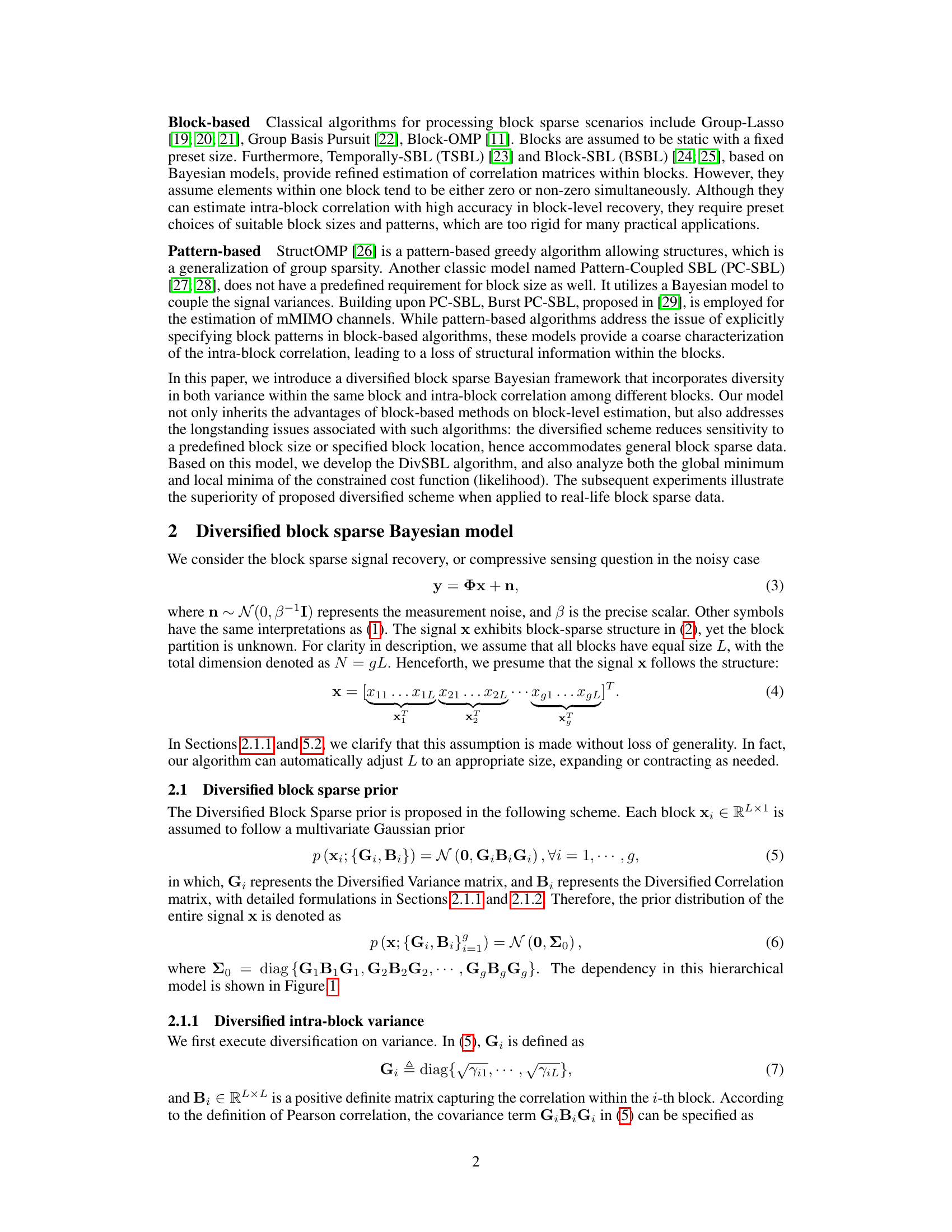
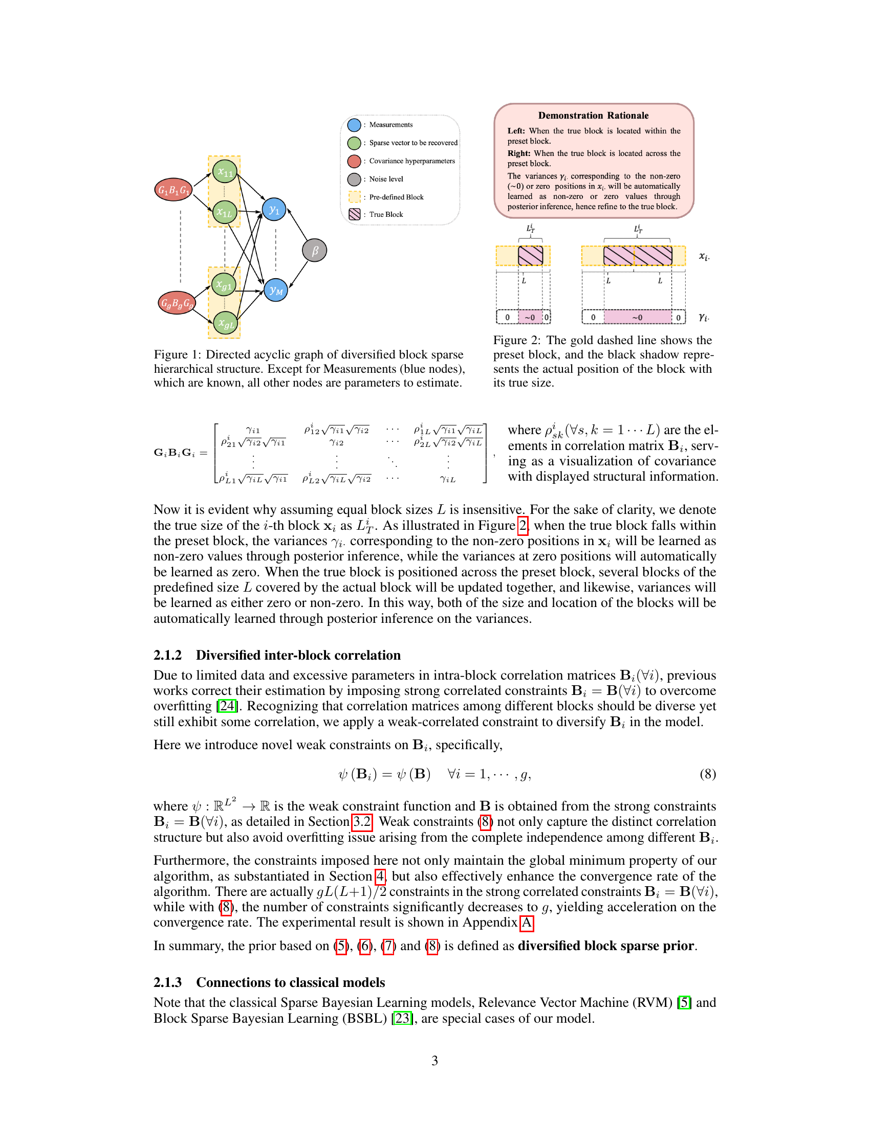
This figure is a directed acyclic graph showing the hierarchical Bayesian model used in the DivSBL algorithm. The nodes represent variables in the model. The blue nodes represent the measurements (y), which are known inputs. The green nodes represent the sparse vector to be recovered (x), which are unknown variables. The red nodes represent the covariance hyperparameters (G, B), which control the prior distribution of the sparse vector. The gray node represents the noise level (β). The yellow dashed boxes represent pre-defined blocks, while the pink dashed boxes represent the true blocks, which the model aims to estimate adaptively. The arrows indicate the dependencies between variables. The model uses a hierarchical Bayesian approach, learning the hyperparameters from the data to estimate the underlying block-sparse structure of the signal.
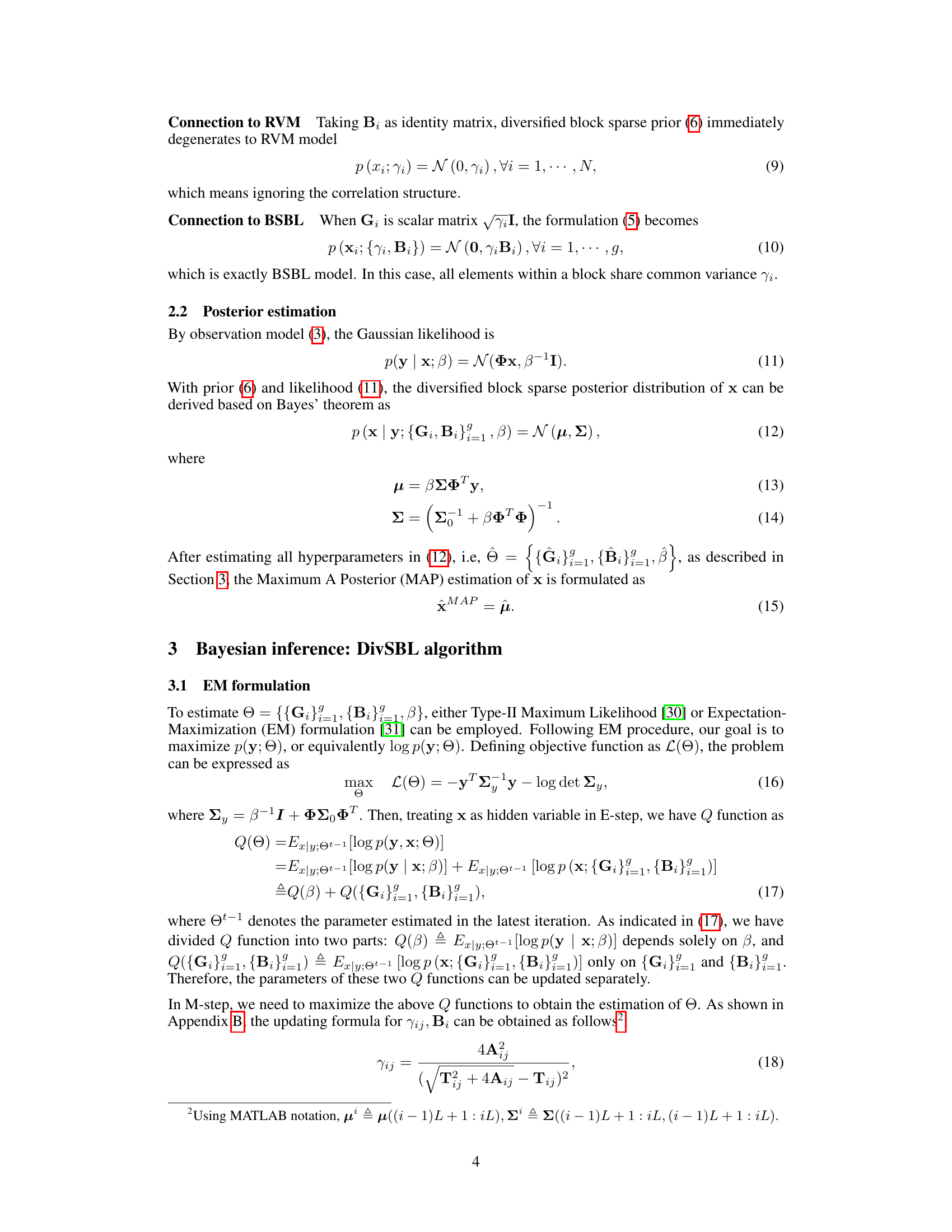
This table presents a comparison of the proposed DivSBL algorithm with other block-sparse and sparse learning algorithms on synthetic datasets. Two scenarios are shown: homoscedastic and heteroscedastic data. For each algorithm, the table shows the Normalized Mean Squared Error (NMSE) and the correlation between the reconstructed and true signals. The NMSE measures the reconstruction error, with lower values indicating better performance, and the correlation measures the similarity in the structure of the reconstructed and true signals, with higher values indicating better performance. DivSBL’s performance is highlighted in blue, and the best results for each metric are bolded.
In-depth insights#
Diversified Block Prior#
The Diversified Block Prior is a novel Bayesian prior designed to model block sparsity in high-dimensional data more effectively than existing methods. Its key innovation lies in its ability to handle both intra-block variance and inter-block correlation in a flexible and adaptive manner. Unlike traditional block sparse priors that assume fixed block sizes and structures, the Diversified Block Prior allows for variation in block sizes and the correlations between blocks, resulting in a more accurate representation of real-world data where block structures are often irregular or unknown. This diversification is achieved through the use of diversified variance and correlation matrices associated with each block, which are then learned from the data. This adaptive approach mitigates the sensitivity of existing block sparse learning methods to pre-defined block structures. By learning the block structures and their variances adaptively, the Diversified Block Prior reduces the risk of overfitting and achieves better performance, particularly in challenging scenarios such as those with limited samples or high noise levels. The efficacy of this approach is demonstrated experimentally through improved signal recovery and reconstruction in comparison to traditional block sparse methods.
DivSBL Algorithm#
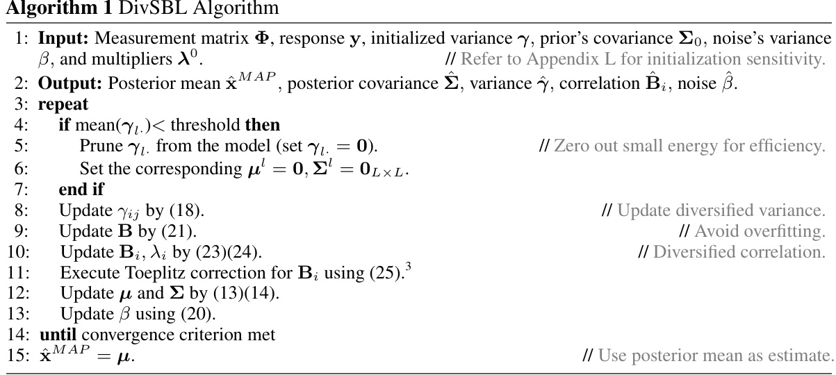
The DivSBL algorithm, a Bayesian approach to block sparse signal recovery, presents a novel solution to overcome limitations of existing methods. Its core innovation lies in the Diversified Block Sparse Prior, which allows for adaptive block estimation by addressing the sensitivity of traditional methods to predefined block structures. This is achieved by introducing diversity in intra-block variance and inter-block correlation matrices, enabling the algorithm to learn the block structure from the data rather than relying on predetermined information. Utilizing the EM algorithm and dual ascent, DivSBL efficiently estimates hyperparameters, further enhancing its adaptability. Theoretically, DivSBL exhibits a global minimum under specific conditions, ensuring accurate recovery, and local minima analysis provides insights into its robustness. Experimental results demonstrate DivSBL’s superiority over existing algorithms, particularly in handling heteroscedastic data and challenging scenarios with varying block sizes. The algorithm’s flexibility and enhanced accuracy make it a significant advancement in block sparse signal recovery for real-world applications.
Global Optimality#
Analyzing the concept of global optimality within the context of a research paper necessitates a deep dive into the methodologies employed to achieve it. The existence of a global optimum is often dependent on specific assumptions and constraints. For instance, the unique representation property (URP) condition, frequently invoked in compressed sensing, ensures a singular solution. However, real-world data rarely adheres perfectly to such idealized conditions. The paper likely explores how these assumptions affect the attainment of a global optimum, potentially highlighting the trade-offs between theoretical guarantees and practical applicability. Furthermore, the computational cost associated with achieving global optimality is a significant consideration. Methods like the Expectation-Maximization (EM) algorithm are widely used, but their convergence to a global solution isn’t always guaranteed. The paper likely offers insights into the balance between computational feasibility and solution quality, potentially outlining a strategy that prioritizes near-optimal solutions over computationally expensive exhaustive searches. The discussion of global optimality, therefore, is pivotal for understanding the algorithm’s robustness and limitations in various real-world scenarios, comparing its performance with other state-of-the-art methods.
Block Size Robustness#
The robustness of block size is a critical aspect of block sparse Bayesian learning algorithms. Traditional methods often struggle with pre-defined block sizes, showing sensitivity to these parameters and yielding suboptimal results when the assumed and true block sizes misalign. A key contribution of diversified block sparse Bayesian learning (DivSBL) is its inherent robustness to variations in block size. DivSBL achieves this through its diversified prior, which allows for adaptive estimation of both the intra-block variance and inter-block correlation. This adaptability effectively mitigates the risk of misspecifying block sizes, thereby ensuring accurate recovery of block sparse signals even when the true block structure is unknown. The experimental results strongly support this claim, showing superior performance compared to existing methods, especially in scenarios with diverse block sizes or when the true size deviates substantially from the pre-defined size. This robustness translates to a more practical and reliable approach for various block sparse signal recovery applications, overcoming limitations of previous algorithms that necessitate precise prior knowledge of the block structure.
Future Research#
Future research directions stemming from this block sparse Bayesian learning method (DivSBL) could explore several promising avenues. Extending DivSBL to handle more complex data structures, such as non-uniform block sizes or hierarchical block structures, would enhance its applicability to diverse real-world datasets. Investigating the impact of different weak correlation constraints on model performance, and developing efficient algorithms for optimizing these constraints, is crucial. Theoretical analysis of the global and local minima of the cost function under more relaxed assumptions, such as non-uniform block sizes or noisy measurements, would strengthen the model’s theoretical foundations. Furthermore, applying DivSBL to a broader range of applications, including those involving high-dimensional data or large-scale datasets, will demonstrate its versatility and practical value. Finally, the exploration of alternative inference methods, such as variational inference or message passing algorithms, could provide computationally efficient alternatives, especially for large-scale problems. Developing scalable DivSBL variants tailored to specific hardware architectures (e.g., GPUs) and investigating its compatibility with emerging hardware could significantly improve performance.
More visual insights#
More on figures
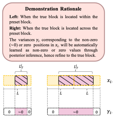
This figure is a directed acyclic graph (DAG) that illustrates the hierarchical Bayesian model used in the proposed DivSBL algorithm. The nodes represent the variables in the model. The blue nodes represent the measurements, which are the observed data. The other nodes represent the parameters to be estimated. The arrows indicate the dependencies between the variables. The figure shows how the different components of the model are related and how they are used to estimate the block sparse signal.

This figure shows a graphical representation of the hierarchical Bayesian model used in the proposed DivSBL algorithm. It illustrates the relationships between different parameters: measurements (y), the sparse vector to be recovered (x), and various hyperparameters (including the diversified variance matrices (Gi), diversified correlation matrices (Bi), and noise level (β)). The arrows indicate the dependencies between the variables. Understanding this graph helps to visualize how the algorithm infers the unknown parameters from the observed measurements.

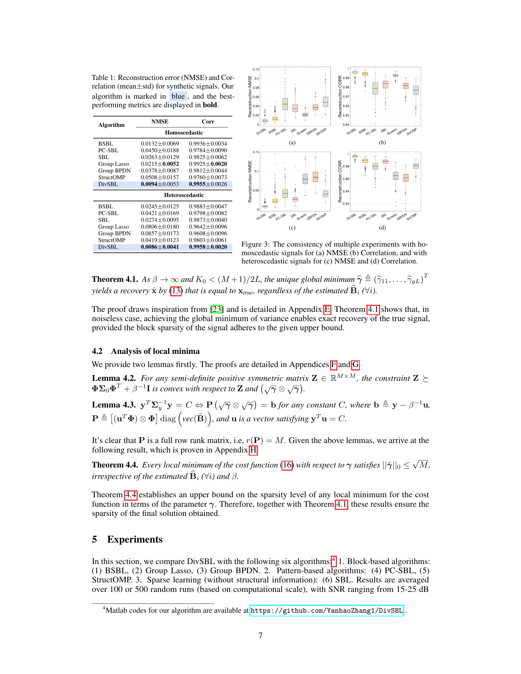
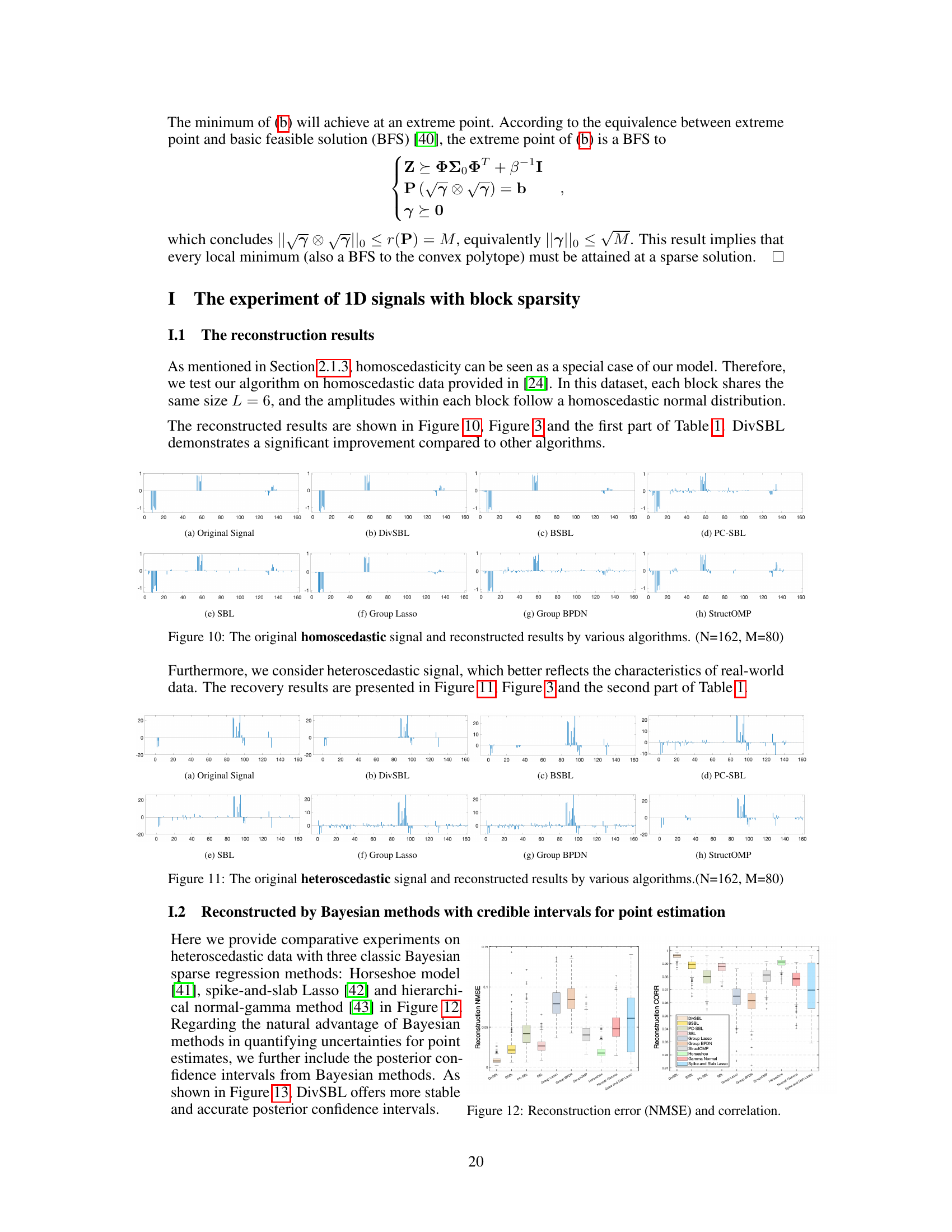
This figure presents the results of multiple experiments to demonstrate the robustness and reliability of the proposed DivSBL algorithm. It shows box plots illustrating the distribution of NMSE (Normalized Mean Squared Error) and correlation values obtained across numerous runs of the experiments, both for homoscedastic and heteroscedastic data. This visual representation helps to quantify the consistency and stability of the DivSBL method compared to other algorithms in recovering the original signals from noisy measurements.

The figure shows box plots of the results of multiple experiments to demonstrate the statistical consistency of the proposed algorithm, DivSBL, compared to other methods (BSBL, PC-SBL, SBL, Glasso, GBPDN, StructOMP) under both homoscedastic and heteroscedastic noise conditions. The plots visualize the distribution of NMSE (Normalized Mean Squared Error) and correlation values, providing a clear comparison of performance across different experimental runs.

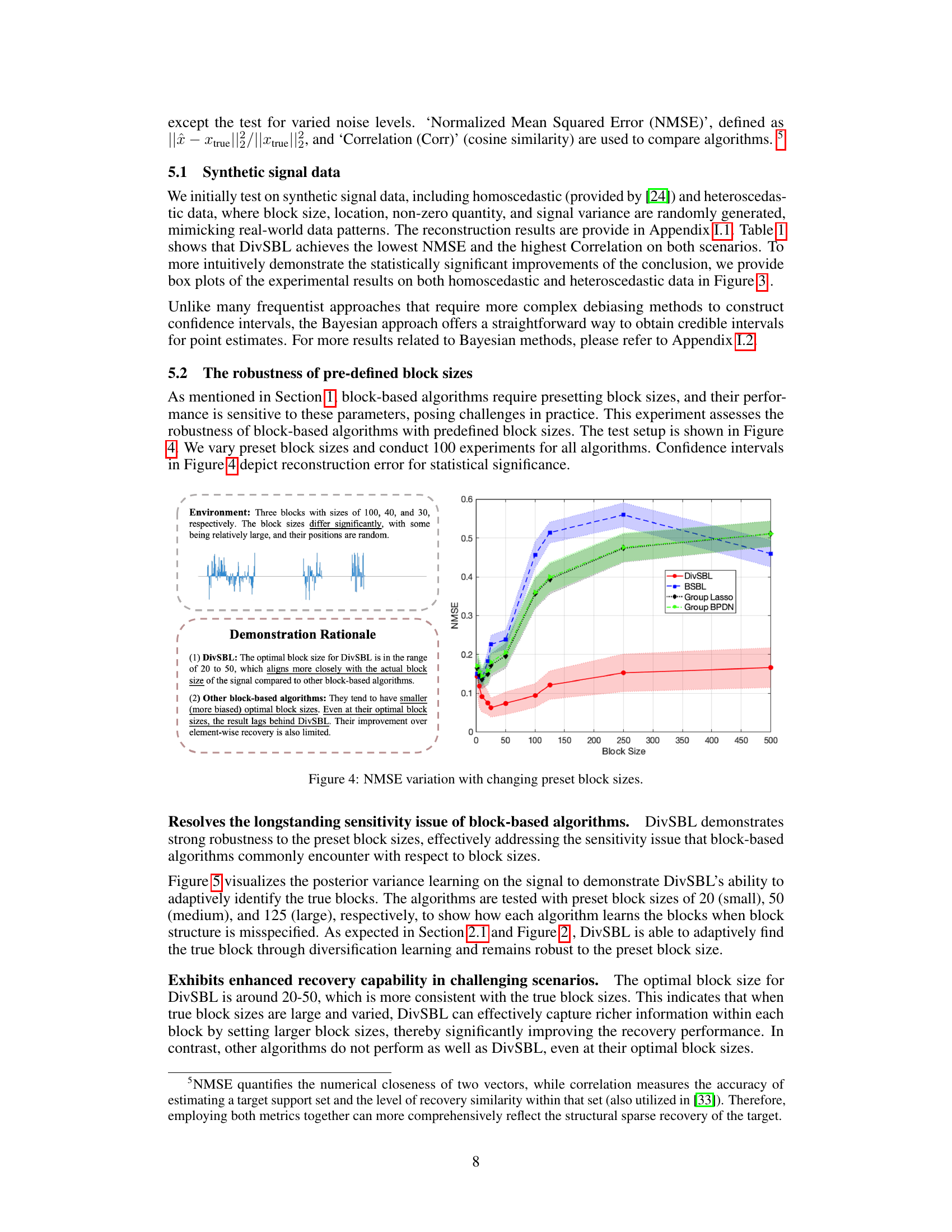
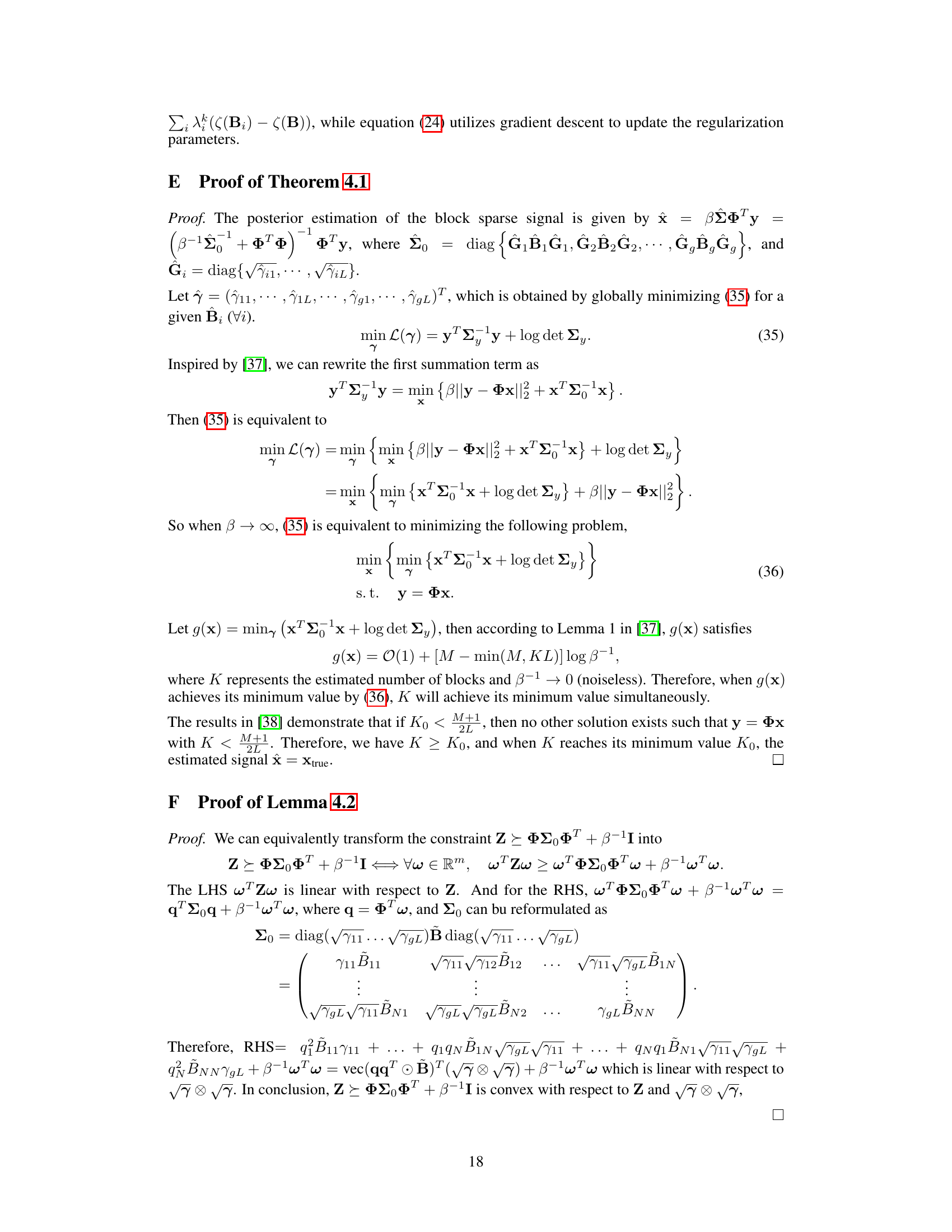
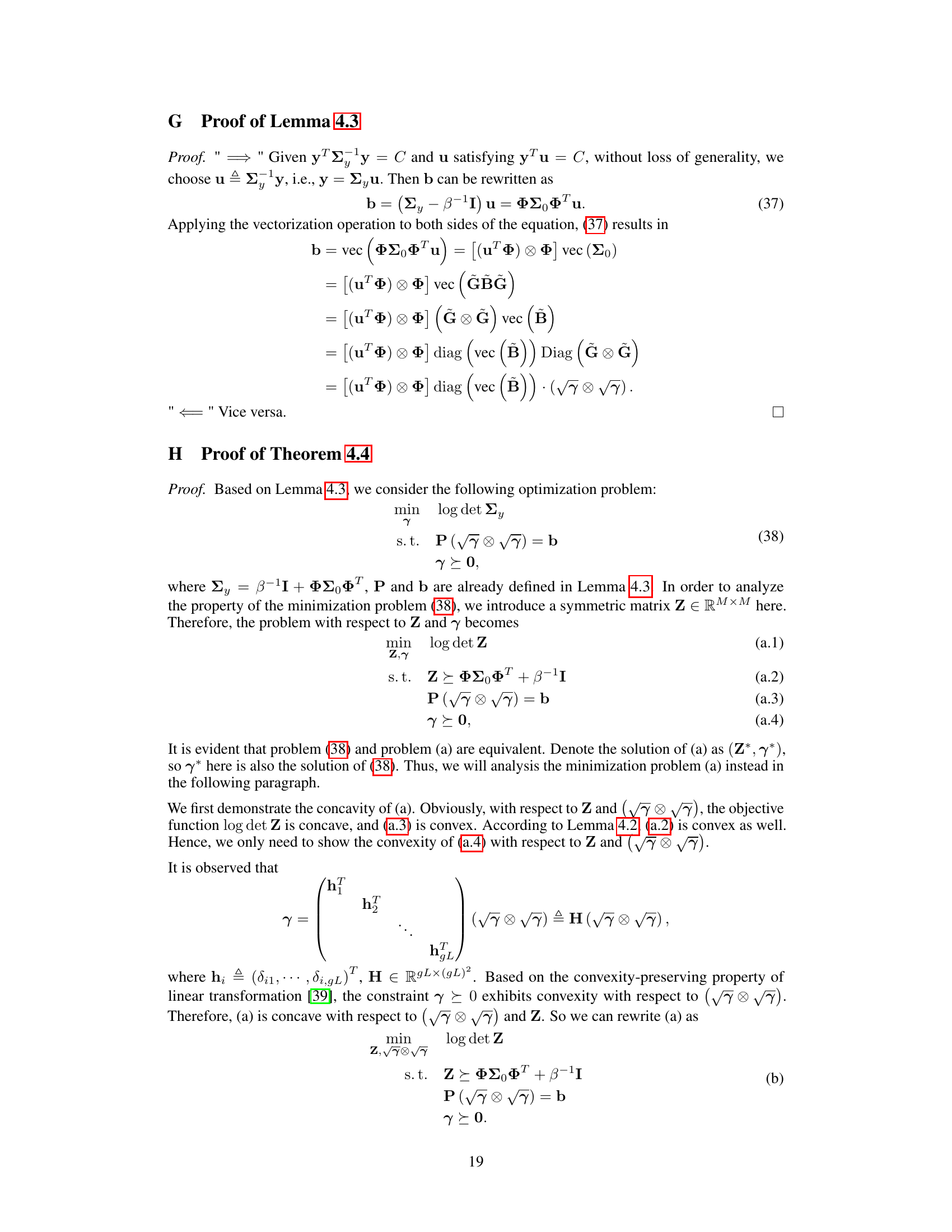
The figure demonstrates the robustness of DivSBL to preset block sizes. It shows that DivSBL consistently achieves lower NMSE (Normalized Mean Squared Error) across a range of preset block sizes, even when those sizes significantly differ from the true block sizes in the signal. In contrast, other block-based algorithms (BSBL, Group Lasso, Group BPDN) show a greater sensitivity to the choice of block size, with performance degrading as the preset block size moves further away from the optimal size. This highlights DivSBL’s superior adaptability in handling block-sparse signals with unknown or variable block structures.
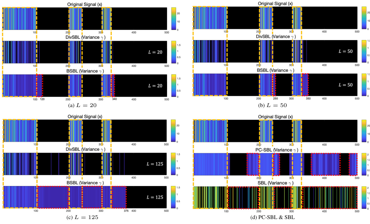
This figure visualizes the posterior variance learning on the signal to demonstrate DivSBL’s ability to adaptively identify the true blocks. The algorithms are tested with preset block sizes of 20 (small), 50 (medium), and 125 (large), respectively, to show how each algorithm learns the blocks when block structure is misspecified. As expected in Section 2.1 and Figure 2, DivSBL is able to adaptively find the true block through diversification learning and remains robust to the preset block size. Exhibits enhanced recovery capability in challenging scenarios. The optimal block size for DivSBL is around 20–50, which is more consistent with the true block sizes. This indicates that when true block sizes are large and varied, DivSBL can effectively capture richer information within each block by setting larger block sizes, thereby significantly improving the recovery performance. In contrast, other algorithms do not perform as well as DivSBL, even at their optimal block sizes.

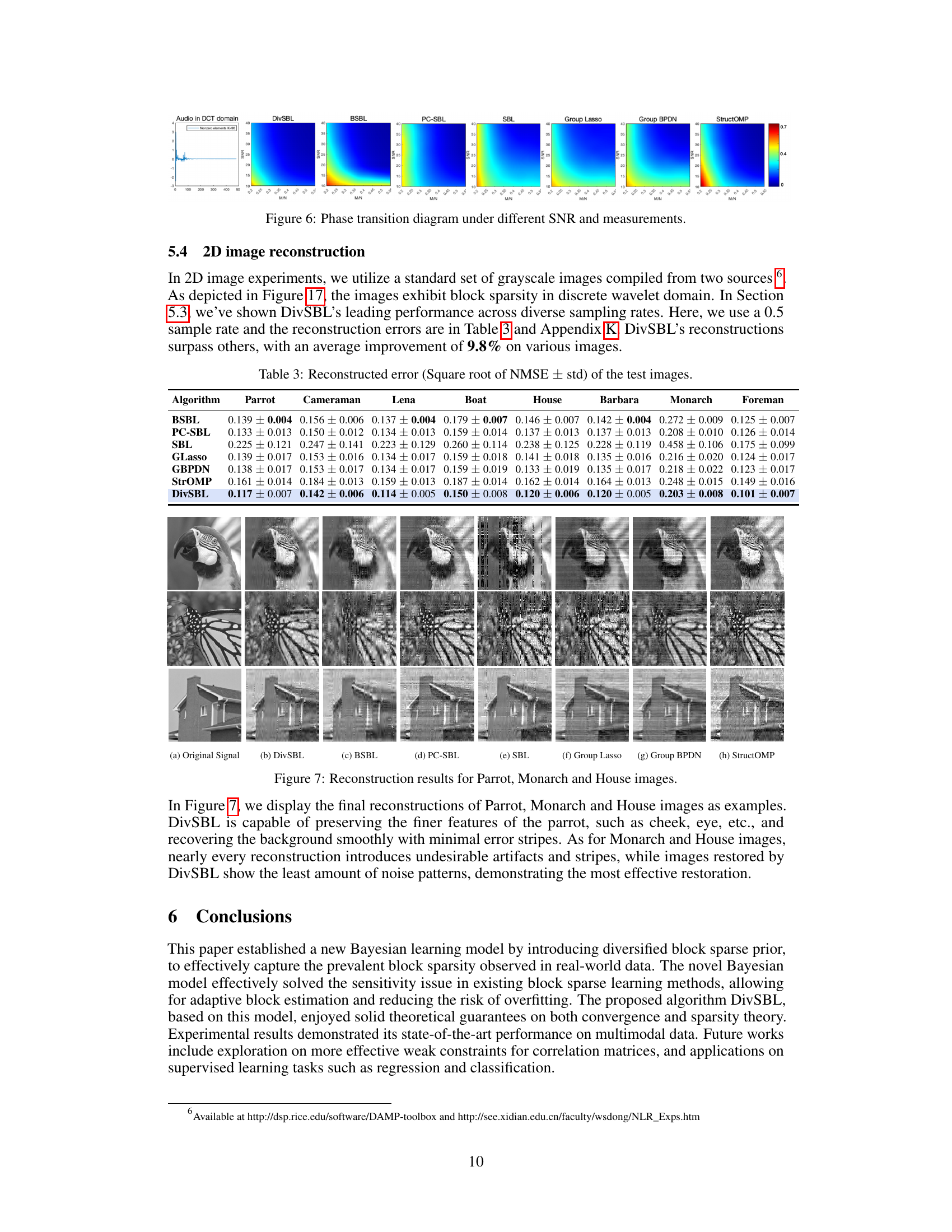
This figure shows the phase transition diagram of DivSBL under various signal-to-noise ratios (SNR) and sampling rates (M/N). It illustrates the algorithm’s performance across different SNR and M/N conditions, showing its robustness and effectiveness in signal recovery. The color intensity represents the NMSE (Normalized Mean Squared Error).

This figure displays the reconstruction results of three images (Parrot, Monarch, and House) using different sparse learning algorithms. The goal is to show the visual quality of the reconstruction. DivSBL is highlighted as offering the best visual reconstruction compared to other methods, preserving finer features and showing minimal artifacts like noise patterns and stripes.
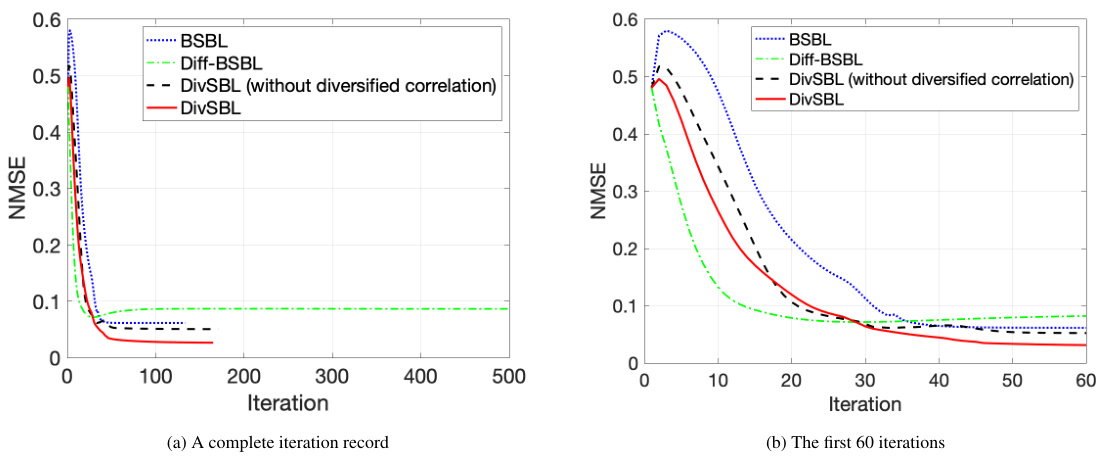
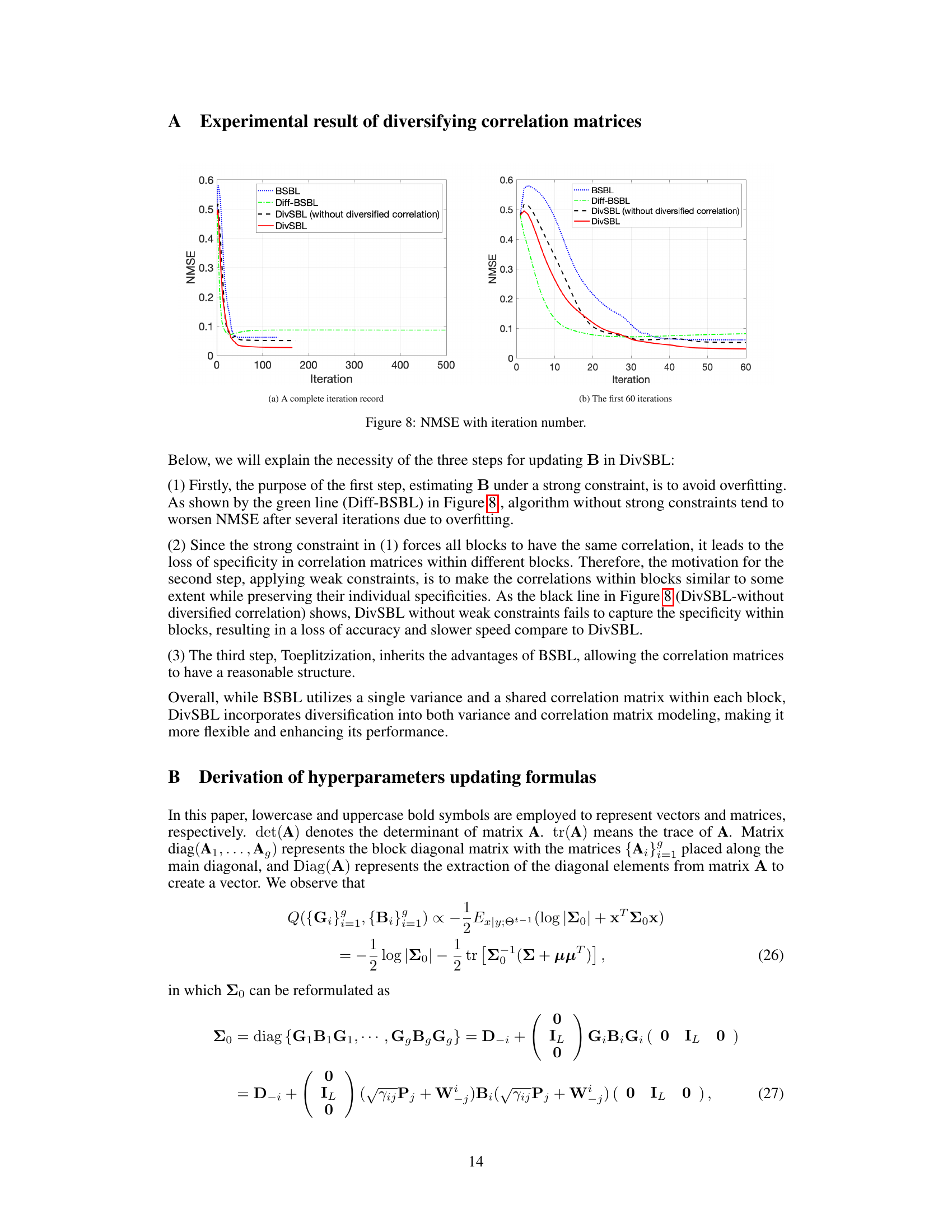
This figure compares the performance of different algorithms in terms of NMSE (Normalized Mean Squared Error) over the number of iterations. It shows the convergence behavior of BSBL (Block Sparse Bayesian Learning), Diff-BSBL (a variation of BSBL), DivSBL (Diversified Block Sparse Bayesian Learning) without diversified correlation, and the proposed DivSBL algorithm. The plot helps to visualize how each algorithm converges to a solution, highlighting the impact of diversified correlation on the speed and accuracy of convergence.
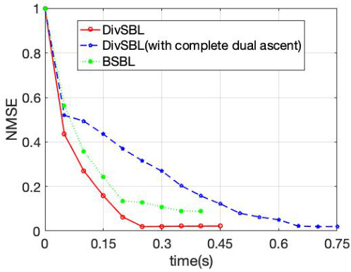
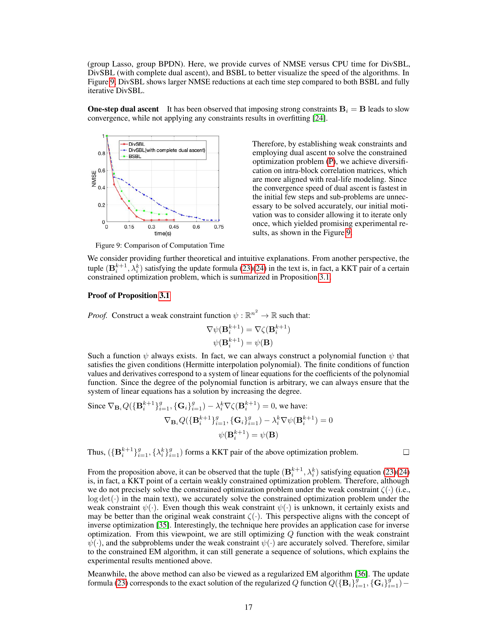
This figure compares the computation time of three algorithms: DivSBL, DivSBL (with complete dual ascent), and BSBL. The x-axis represents the CPU time (in seconds), and the y-axis represents the NMSE. It demonstrates that DivSBL achieves faster NMSE reduction compared to both BSBL and the fully iterative DivSBL.

This figure shows the hierarchical Bayesian model used in the Diversified Block Sparse Bayesian Learning (DivSBL) method. It illustrates the relationships between different parameters in the model. The blue nodes represent the observed measurements (y), which are known. The other nodes represent the parameters that need to be estimated: the sparse vector to be recovered (x), the intra-block variance (G), the inter-block correlation (B), and the noise level (β). The arrows indicate the dependencies between the parameters. The figure visually represents the hierarchical structure of the model.

This figure shows a directed acyclic graph (DAG) illustrating the hierarchical Bayesian model used in the Diversified Block Sparse Bayesian Learning (DivSBL) method. The DAG depicts the relationships between various parameters in the model, including the observed measurements (y), the sparse signal (x) to be recovered, and hyperparameters representing the diversified variance (G), diversified correlation (B), and noise level (β). The nodes represent the variables, and the arrows indicate the dependencies between them.

This figure demonstrates the reliability of the experimental results by showing box plots for multiple experimental runs under both homoscedastic and heteroscedastic noise conditions. The plots visualize the distribution of NMSE and Correlation values across various trials, showcasing the algorithm’s consistent performance and highlighting the statistical significance of the findings.

The figure displays the posterior mean and credible intervals for each of the six algorithms considered in the paper: DivSBL, BSBL, PC-SBL, SBL, Horseshoe, and Normal-Gamma. The credible intervals visualize the uncertainty associated with the point estimates. It helps to understand the stability and accuracy of the posterior estimates for different methods.

The figure shows the original audio signal and its sparse representation after applying Discrete Cosine Transform (DCT). The original signal (a) is a continuous waveform. After DCT transformation, it exhibits a block-sparse structure, meaning that non-zero elements in the transformed signal appear in clusters (b). This illustrates the block sparsity phenomenon used as a basis for the DivSBL algorithm, which is designed to handle this specific structure for enhanced signal recovery.

This figure shows a graphical representation of the hierarchical Bayesian model used in the Diversified Block Sparse Bayesian Learning (DivSBL) method. It illustrates the dependencies between different model parameters, including the measurements, the sparse vector to be recovered, the diversified variance and correlation matrices, and the noise level. The nodes represent the parameters, and the arrows indicate the dependencies between them, showing how each parameter is used to estimate other parameters in a hierarchical fashion. This visualization aids understanding the complex relationship between the different components of the DivSBL model.
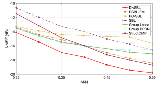
This figure shows the NMSE (Normalized Mean Squared Error) performance of DivSBL and other algorithms across different sampling rates (M/N). The x-axis represents the sampling rate, and the y-axis represents the NMSE in dB. DivSBL consistently outperforms other methods across all sampling rates, demonstrating its robustness and efficiency in recovering signals with varying levels of sampling.
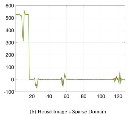
This figure displays the first five columns of the sparse representation of Parrot and House images in the discrete wavelet domain. The plots visualize the wavelet coefficients after the image data has undergone a discrete wavelet transform, revealing a block-sparse structure where non-zero coefficients are clustered together.

This figure shows the sparse representation of Parrot and House images in the discrete wavelet domain. The first five columns of the transformed data are displayed. This visualization helps to illustrate the block sparsity structure present in the images, which is a key characteristic exploited by the DivSBL algorithm for improved reconstruction.

This figure demonstrates the consistency and reproducibility of the experimental results by showing box plots of NMSE and correlation for multiple experiments. The plots are separated into homoscedastic and heteroscedastic signal cases, providing a clear visual representation of the performance variability across different runs. The consistency of the results across various trials strengthens the conclusions made by the authors regarding the superior performance of their proposed approach.
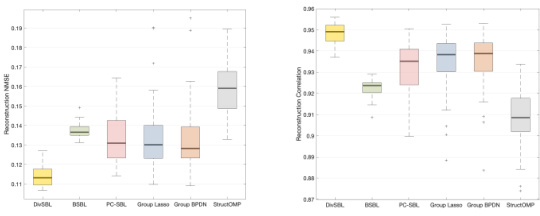
This figure demonstrates the consistency and reliability of the DivSBL algorithm’s performance across multiple experimental runs. The results are presented in box plots for both homoscedastic and heteroscedastic synthetic signals. Each box plot shows the distribution of NMSE and correlation values obtained across the various runs. The consistency of the results across multiple runs and the different types of signals (homoscedastic and heteroscedastic) validates the algorithm’s robustness and effectiveness.
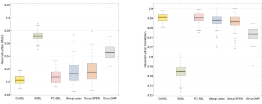
This figure demonstrates the robustness and consistency of the proposed DivSBL algorithm across multiple experimental runs. It displays box plots visualizing the distribution of NMSE (Normalized Mean Squared Error) and Correlation values obtained for both homoscedastic and heteroscedastic synthetic signal data. The consistent performance across multiple runs highlights the reliability and stability of DivSBL in different scenarios.
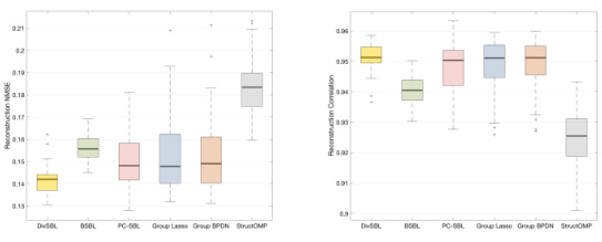
This figure demonstrates the consistent performance of the DivSBL algorithm across multiple experimental runs. It shows box plots illustrating the distribution of NMSE (Normalized Mean Squared Error) and correlation values obtained for both homoscedastic (consistent variance) and heteroscedastic (varying variance) synthetic signals. The results demonstrate that DivSBL consistently outperforms other algorithms in terms of both reconstruction accuracy (lower NMSE) and correlation with the true signal.
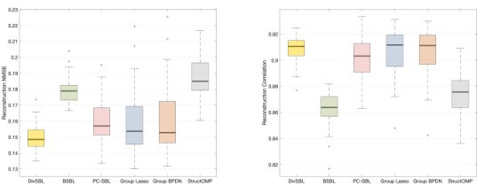
This figure displays box plots visualizing the consistency of the results obtained from multiple experiments. The left panel shows results for homoscedastic signals, and the right panel shows results for heteroscedastic signals. Each panel presents two subplots: (a) and (c) show the Normalized Mean Squared Error (NMSE), while (b) and (d) show the correlation. The box plots summarize the NMSE and correlation values from multiple experimental runs, providing a visual representation of the distribution and variability of the results across different runs, for both homoscedastic and heteroscedastic data.
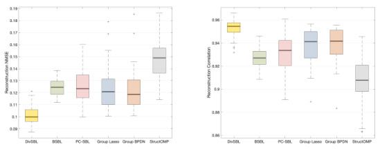
The figure shows box plots for the results of multiple experiments performed on both homoscedastic and heteroscedastic signals to confirm the reliability of the results. The NMSE (Normalized Mean Squared Error) and Correlation are used as evaluation metrics. The plots display the distribution of NMSE and Correlation values for each algorithm across multiple experimental runs, illustrating the consistency and statistical significance of the findings.

This figure presents the results of multiple experiments conducted to evaluate the performance of the proposed DivSBL algorithm and other competing algorithms. The experiments were carried out using both homoscedastic (consistent variance) and heteroscedastic (variable variance) synthetic signals. The figure displays box plots showing the distribution of NMSE (Normalized Mean Squared Error) and Correlation values obtained across these multiple runs. This visualization demonstrates the robustness and consistency of DivSBL’s performance compared to the other methods under different signal characteristics.
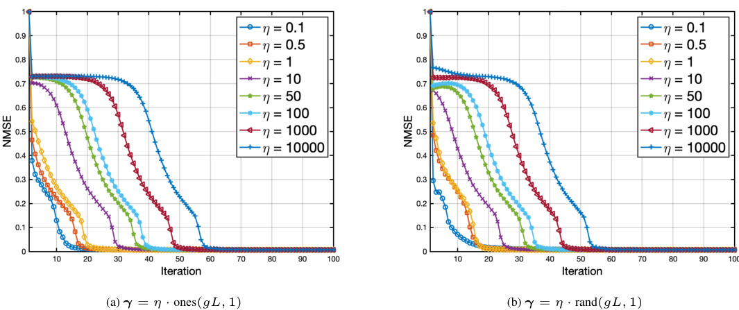
This figure displays the sensitivity analysis of the DivSBL algorithm to the initialization of variance parameters (γ). Two initialization methods are used: (a) γ = η * ones(gL, 1) and (b) γ = η * rand(gL, 1), where η is a scaling factor that varies across different values (0.1, 0.5, 1, 10, 50, 100, 1000, 10000). The NMSE (Normalized Mean Squared Error) is plotted against the iteration number for each η value. The results show that although different initializations of γ affect the convergence speed to some extent, the algorithm converges to a similar NMSE value in all cases, indicating its robustness to initialization choices.
More on tables
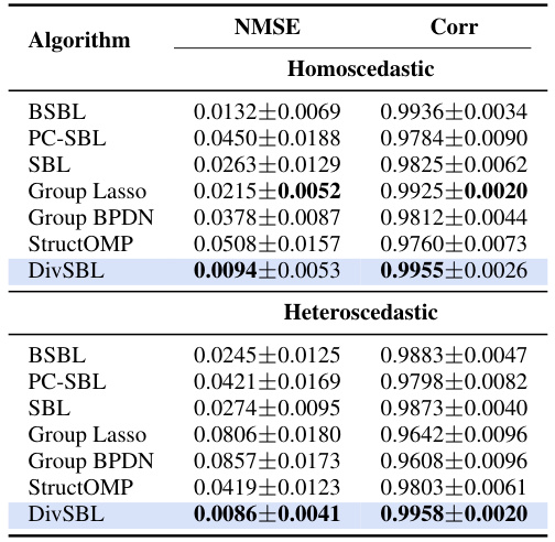
This table presents the results of reconstruction error (NMSE) and correlation for both homoscedastic and heteroscedastic synthetic signals. The NMSE (Normalized Mean Squared Error) measures the difference between the reconstructed signal and the true signal. The correlation measures the similarity between the reconstructed and true signals. The table compares the proposed DivSBL algorithm against several other block-sparse and sparse learning algorithms. The best performing algorithm for each metric (lowest NMSE and highest correlation) is highlighted in bold. DivSBL is shown in blue.

This table presents the reconstruction errors, specifically the Normalized Mean Squared Error (NMSE) along with their standard deviations, obtained from experiments conducted on audio signals at a sample rate of 0.25. The results are categorized based on different Signal-to-Noise Ratios (SNR) ranging from 10 to 50. Each SNR level includes results from multiple algorithms: BSBL, PC-SBL, SBL, Group BPDN, Group Lasso, StructOMP, and DivSBL. The table helps to assess the performance and robustness of these algorithms under various noise conditions.

This table presents the results of reconstruction error (measured by NMSE) and correlation for synthetic signals using different algorithms. The algorithms compared include DivSBL (the proposed method), BSBL, PC-SBL, SBL, Glasso, GBPDN, StrOMP, Group Lasso, and Group BPDN. Two types of synthetic signals are used: homoscedastic and heteroscedastic. The best performing algorithm for each metric is shown in bold, highlighting the superiority of DivSBL.
Full paper#

