↗ OpenReview ↗ NeurIPS Homepage ↗ Chat
TL;DR#
Optimal transport (OT) aims to efficiently map one probability distribution to another. Standard OT methods often use squared Euclidean distance as a cost function, which can be problematic in high dimensions. This paper tackles this challenge by exploring ’elastic costs,’ which incorporate a regularizer to shape the displacements of the transport map, effectively reducing the dimensionality of the problem. The main difficulty lies in the computational burden and the lack of tools to study these problems.
This paper proposes a novel numerical method to compute optimal Monge maps for elastic costs, enabling the generation of synthetic datasets with known ground-truth maps. It then introduces ‘subspace elastic costs,’ which promote displacements within low-dimensional subspaces. To effectively learn the parameters of these subspace costs, it proposes a bilevel loss function. Experiments on synthetic and single-cell data demonstrate improved predictive ability of subspace elastic costs compared to conventional methods. This research contributes both practically through improved computational efficiency and improved prediction performance and theoretically with the introduction of new tools and the analysis of the statistical properties of the MBO estimator with subspace elastic costs.
Key Takeaways#
Why does it matter?#
This paper is important because it introduces a novel method for learning optimal transport maps with structured displacements. It addresses the limitations of standard cost functions in high-dimensional settings by using elastic costs and a bilevel loss function. This opens up new avenues for research in optimal transport, with applications in various fields such as single-cell genomics and machine learning. The work is also important for its theoretical contributions, proving the consistency of the proposed estimator and providing new insights into the statistical properties of optimal transport maps. The provided numerical scheme is also a significant contribution, which will help further research of optimal transport problems.
Visual Insights#

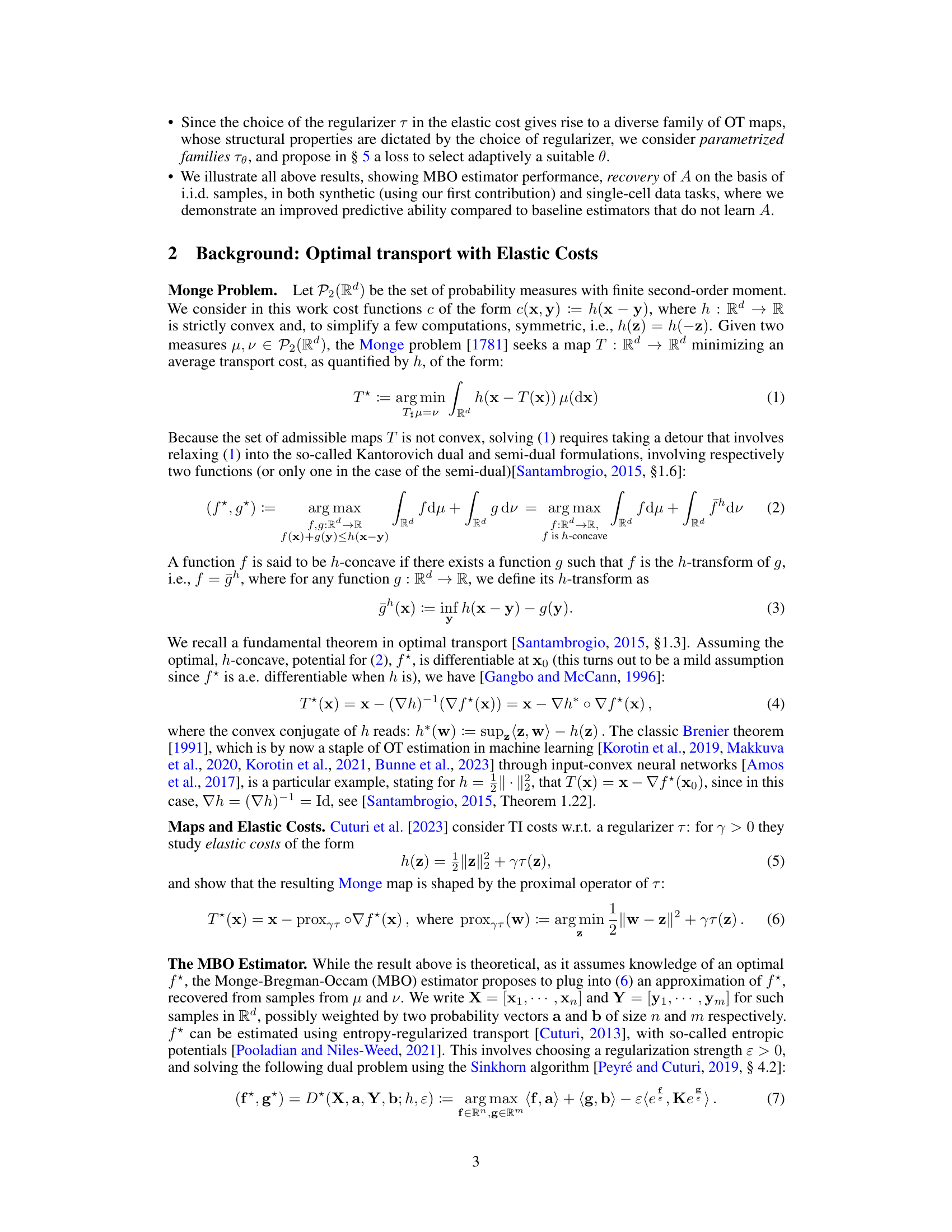
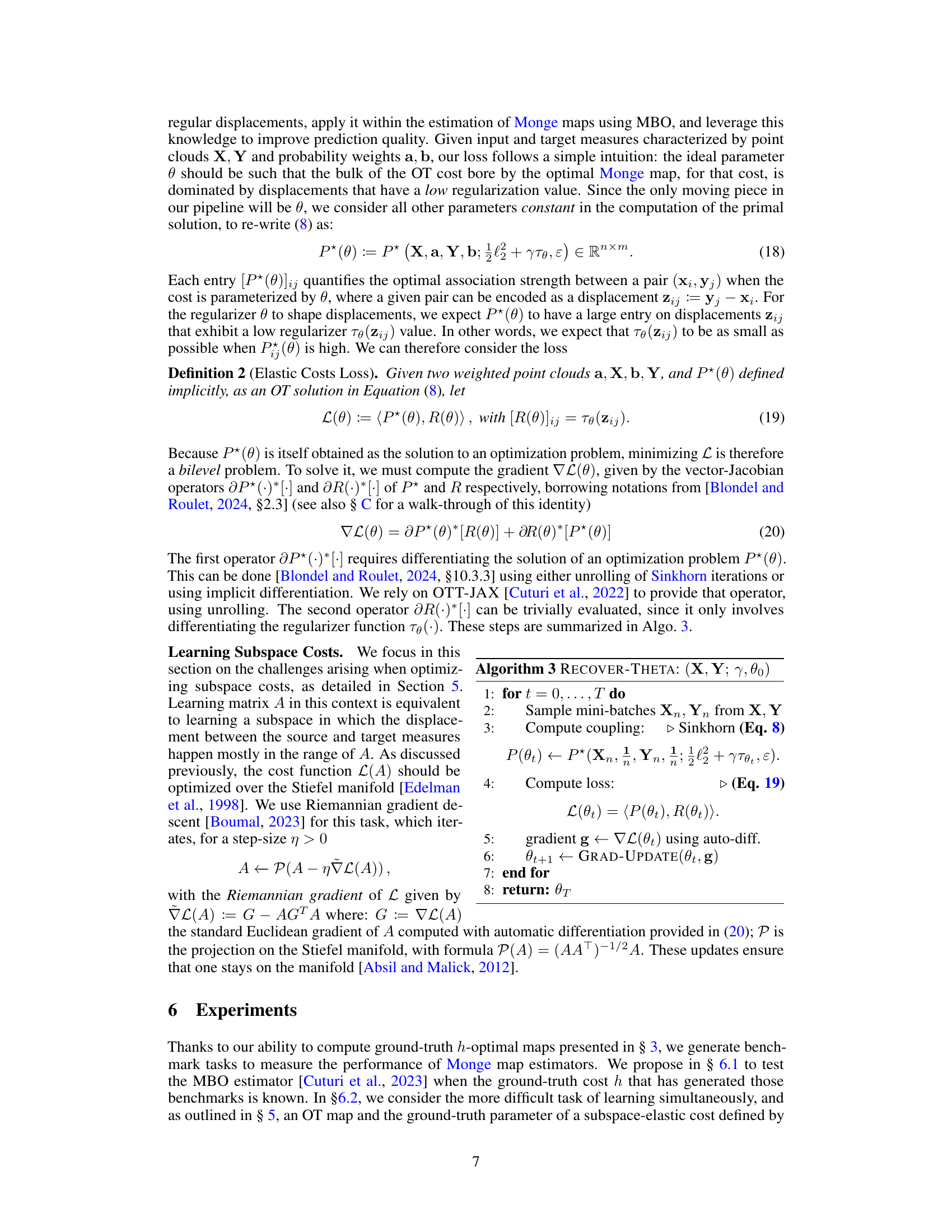
This figure shows four examples of optimal transport maps with different cost functions (h). Each example uses the same base function (g), which is visualized by its level lines. The differences in the maps illustrate how the choice of cost function influences the structure of the resulting transport map. Different costs induce different patterns of displacements, ranging from smooth (l2 cost) to sparse (l1 cost) and directional (cost that penalizes displacements orthogonal to vector b).

This table shows the number of cells used in the single-cell RNA sequencing experiment for each cell line (A549, K562, MCF7) and for each drug or control condition (Control, Dac, Giv, Bel, Hes, Quis). These numbers are important because they represent the sample sizes for each group in the analysis, influencing the statistical power and reliability of the results.
In-depth insights#
Elastic Cost in OT#
The concept of “Elastic Costs in Optimal Transport” introduces a regularization to the traditional cost function in OT, moving beyond the typical squared Euclidean distance. This regularization, often denoted by a term γτ(x-y), where γ is a hyperparameter and τ is a regularizer function, shapes the resulting Monge map by influencing the displacements between source and target points. The regularizer, τ, imposes structure on the map’s displacements, potentially promoting sparsity, low-dimensionality, or other desirable properties. Key benefits include improved estimation of OT maps in high-dimensional spaces, where the curse of dimensionality is a significant challenge, and the ability to incorporate prior knowledge about the underlying data structure. The selection of the regularization hyperparameter, γ, and the choice of the regularizer function, τ, significantly impacts the resulting map, offering flexibility in tailoring OT solutions to specific applications. A critical aspect is that the choice of regularizer guides the structure of the resulting transport map, creating a link between the proximal operator of the regularizer and the structure of the Monge map’s displacements. This enables researchers to design custom cost functions promoting specific structures, leading to more interpretable and effective OT solutions.
MBO Map Estimator#
The Monge-Bregman-Occam (MBO) map estimator offers a novel approach to computing optimal transport (OT) maps, particularly useful for high-dimensional data. It leverages the concept of elastic costs, which incorporate a regularizer into the standard cost function, shaping the resulting OT map and mitigating the curse of dimensionality. The MBO estimator is computationally efficient, employing proximal gradient descent methods which are easily adapted to various cost functions. A key advantage is the ability to learn cost parameters adaptively, which allows for tailoring OT maps to specific data structures, significantly improving predictive performance in scenarios like single-cell genomics. While the algorithm’s statistical consistency has been shown, there are opportunities for exploring the effects of different regularizers and investigating theoretical guarantees for more complex situations. The method is a promising step towards more robust and effective OT map estimation in high-dimensional applications.
Subspace Elastic Costs#
The concept of “Subspace Elastic Costs” introduces a novel regularization technique within the framework of optimal transport (OT). It addresses the computational challenges of high-dimensional OT by promoting displacement vectors to reside within a lower-dimensional subspace. This is achieved by incorporating a regularizer that penalizes displacements orthogonal to the chosen subspace, effectively reducing the dimensionality of the problem. The core idea is to learn this subspace from data, enabling the model to focus on relevant variations while ignoring noise. This technique offers significant computational advantages in high-dimensional settings and has potential to improve prediction accuracy by incorporating prior knowledge or structure within the data. The effectiveness of the approach is validated through theoretical analysis and empirical evaluation on both synthetic and real-world single-cell data, demonstrating the ability to learn the optimal subspace and improve model performance.
Bilevel Loss Function#
A bilevel loss function, in the context of learning optimal transport (OT) maps with elastic costs, presents a novel approach to learning the parameters of a regularizer within an OT framework. The core idea is to optimize a cost function (upper level) that depends on the solution of an optimal transport problem (lower level). The lower level involves solving for the optimal transport plan using a parameterized cost function, and the upper level aims to optimize the parameters of this cost function. This bilevel structure elegantly addresses the challenge of learning the regularizer by directly linking its parameters to the characteristics of the optimal transport maps. The upper-level loss function is designed to encourage transport maps with desirable properties, such as sparsity or low-dimensionality. This is achieved by penalizing the magnitude of the regularizer’s output for highly weighted transport pairings. Efficient optimization strategies are essential for training such bilevel models, potentially involving techniques like gradient descent on the upper level and an appropriate solver (such as Sinkhorn) for the lower level. Although the computation is more complex than typical single-level optimization, the bilevel approach’s ability to directly shape the resulting OT map through parameter learning is a significant advantage, promising improved predictive performance in applications involving high-dimensional data.
Future Work#
The research paper’s “Future Work” section would ideally explore several promising avenues. Extending the subspace elastic cost framework to more general cost functions and regularizers beyond the specific choices explored is crucial for broader applicability. Investigating the theoretical properties, particularly regarding sample complexity and convergence rates, with a deeper focus on high-dimensional settings, is vital for solidifying the method’s statistical foundation. Addressing the computational challenges inherent in handling high-dimensional data is also key, possibly by investigating more efficient optimization algorithms or leveraging techniques like dimensionality reduction. Empirically, applying the learned elastic costs to a wider array of datasets, such as those involving time series or complex biological networks, would demonstrate the method’s robustness and versatility across diverse application domains. Finally, developing a more principled way to automatically select the optimal subspace dimension rather than relying on pre-specified values would further enhance the method’s practicality and interpretability.
More visual insights#
More on figures

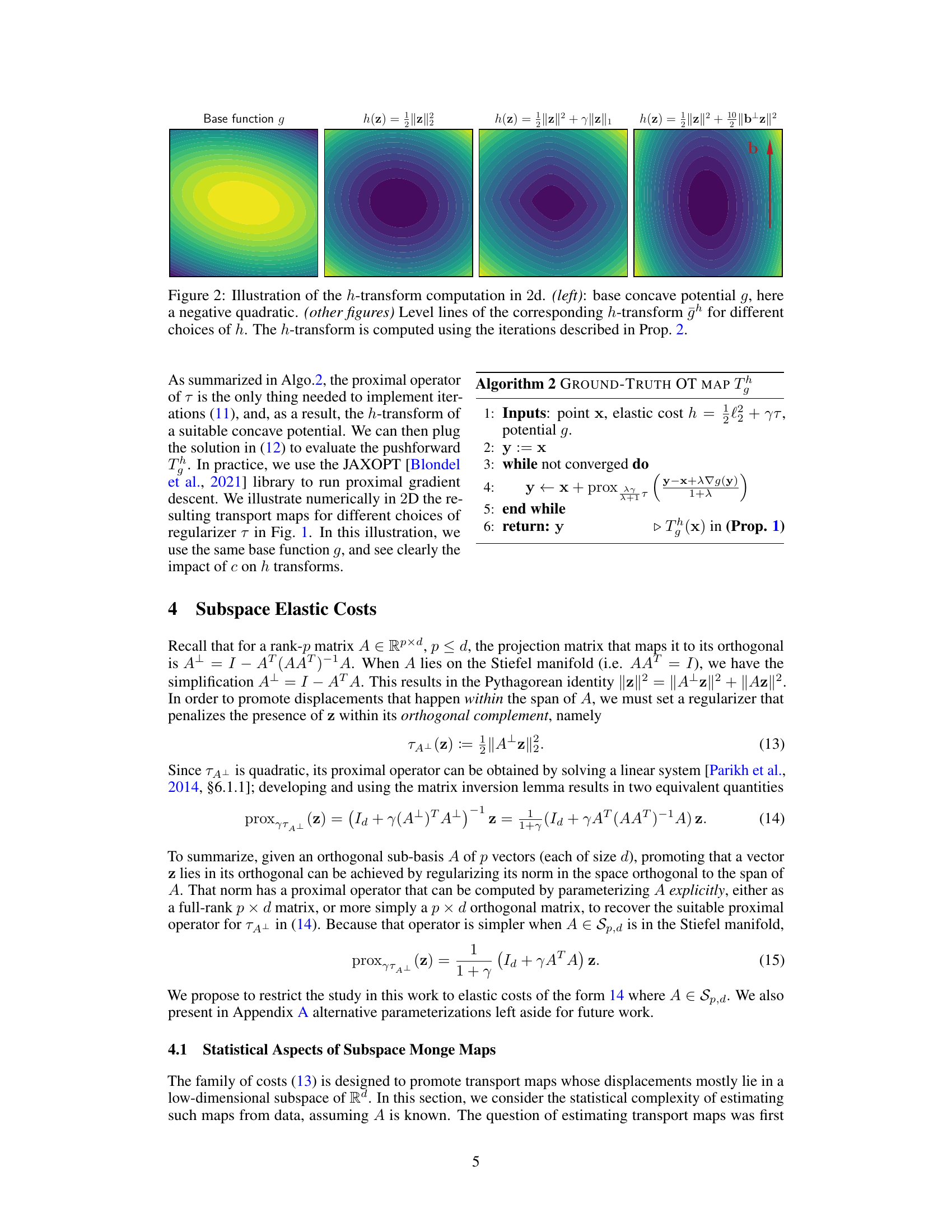
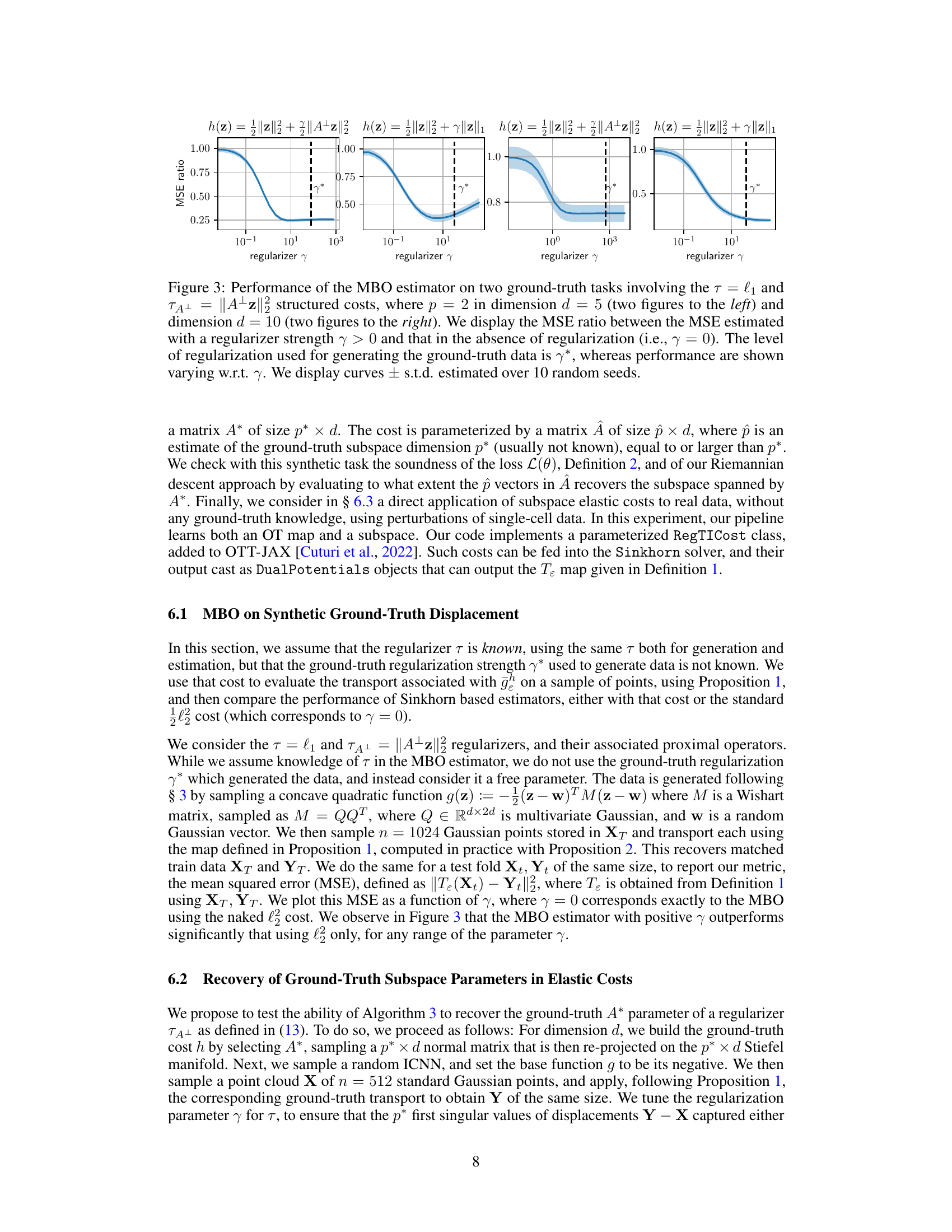
This figure shows the computation of the h-transform for different cost functions (h). It starts with a base concave potential function g (a negative quadratic in this case) and then computes the h-transform using the iterative method described in Proposition 2. The figure displays the level lines of the h-transform for each of the four cost functions considered. Different cost functions lead to substantially different h-transforms, and, as a consequence, the optimal transport maps for those costs.

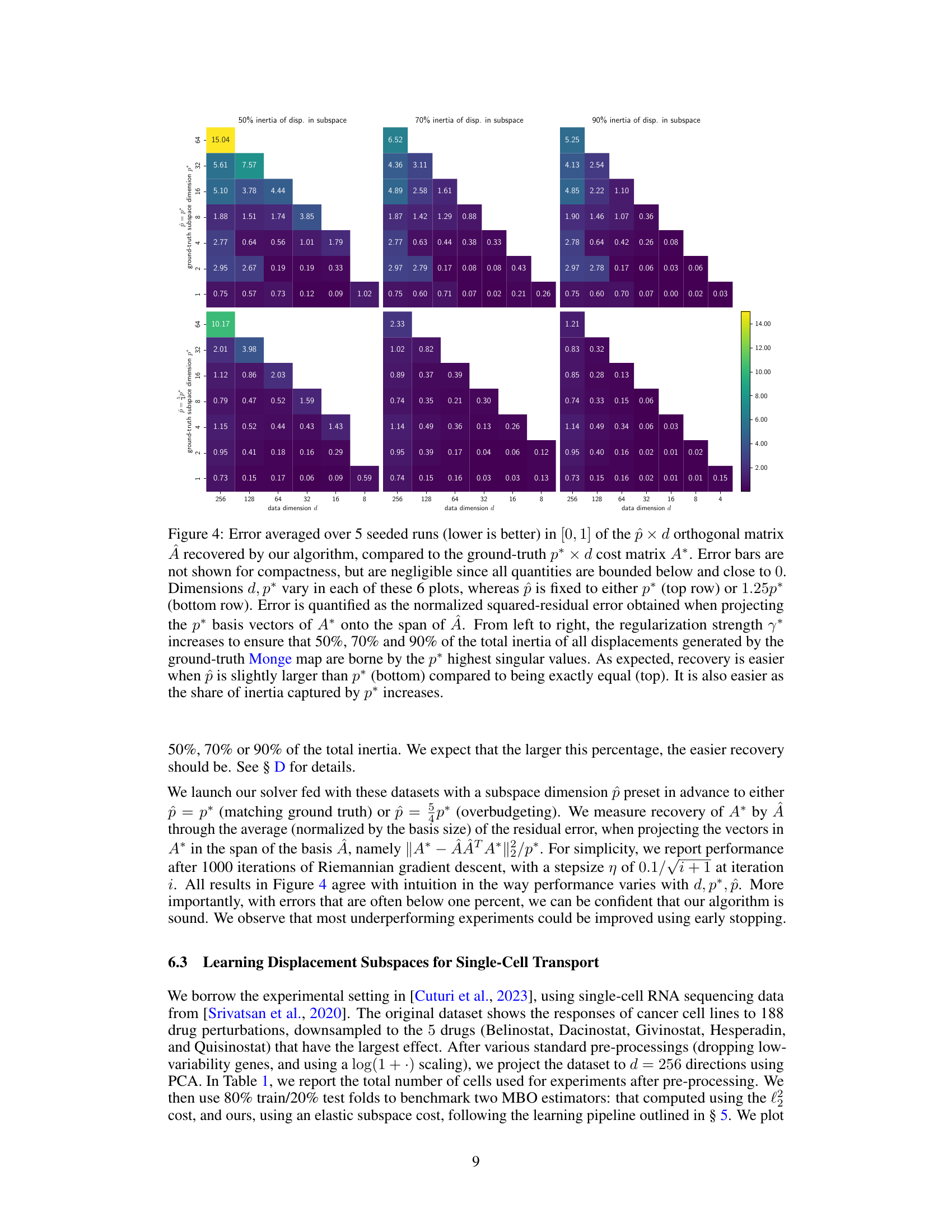
The figure displays the performance of the Monge-Bregman-Occam (MBO) estimator on synthetic datasets. Two different regularizers (l1 and ||A+z||2) are used in two different dimensions (d=5 and d=10). The Mean Squared Error (MSE) ratio (with regularization vs. without) is plotted against various regularization strength (γ), showing improved performance with appropriate regularization, especially in higher dimensions.
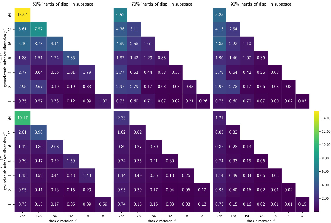
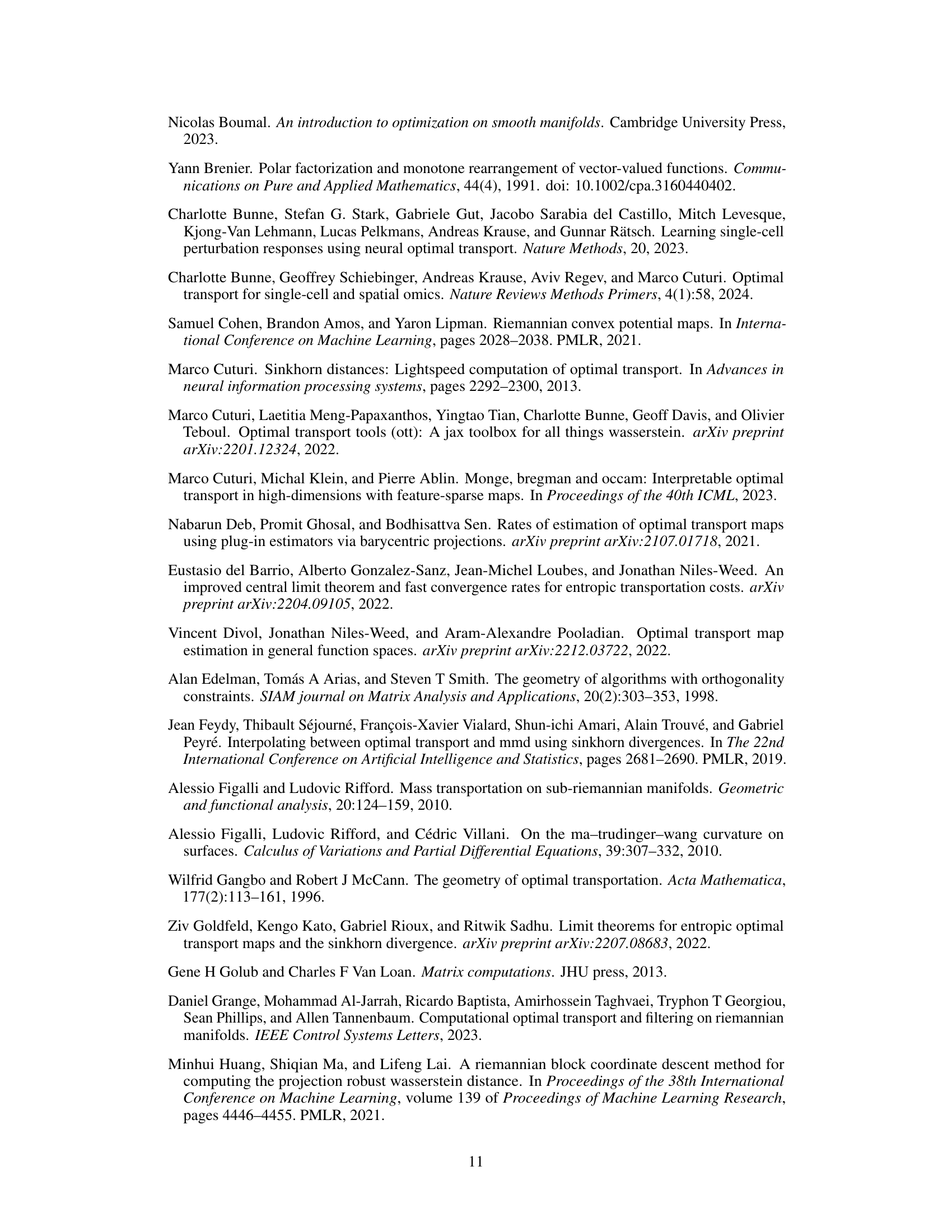
This figure displays the results of an experiment evaluating the ability of the algorithm to recover the ground truth subspace parameters in elastic costs. It shows the error in recovering a low-dimensional subspace (represented by matrix A) using different dimensions for the data (d), the true subspace (p*), and the estimated subspace (p̂). The experiment was conducted with varying percentages (50%, 70%, 90%) of inertia of displacements in the true subspace, and the results indicate improved recovery performance with higher inertia percentages and slightly overestimated subspace dimensions.

This figure displays the predictive performance of the Monge-Bregman-Occam (MBO) estimator on single-cell datasets with 256 dimensions. It compares the performance using the standard l2 cost with that of the elastic subspace cost. The results show that promoting displacements within a lower-dimensional subspace significantly improves predictive performance, even when evaluating using the squared Euclidean distance. The x-axis represents varying values of the regularization parameter (γ), and the different colored lines indicate varying subspace dimensions (p).
More on tables
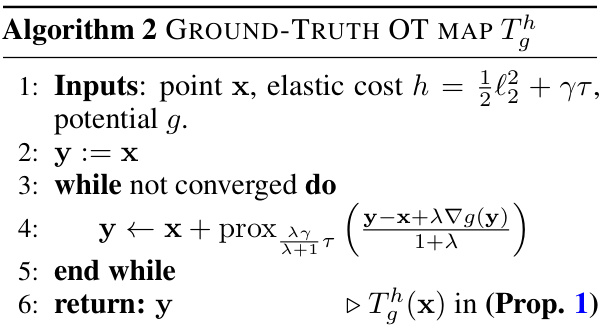
This table shows the number of cells used in each cell line for the control group and for each of the five drugs (Belinostat, Dacinostat, Givinostat, Hesperadin, and Quisinostat). These cell counts are used in the single-cell RNA sequencing experiments described in Section 6.3 of the paper.
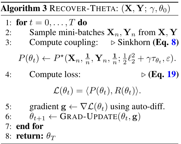
This table shows the number of cells used in the single-cell RNA sequencing experiment for each cell line (A549, K562, MCF7) and treatment group (control, Belinostat, Dacinostat, Givinostat, Hesperadin, Quisinostat). These numbers represent the sample sizes used for the downstream analysis and predictive performance evaluation of the optimal transport methods.

This table shows the number of cells used in the single-cell RNA sequencing experiment for each of the three cell lines (A549, K562, MCF7) and for each of the six drug/control conditions (Control, Dac, Giv, Bel, Hes, Quis). These numbers represent the sample sizes used in the downstream analysis for each condition.

This table shows the number of cells for each cell line and drug/control splits used in the single-cell RNA sequencing data experiments described in Section 6.3. The data comes from the Srivatsan et al. (2020) dataset, which was downsampled to only include the five drugs with the largest effects. The table provides context for the experimental results on single-cell data.
Full paper#

